Jonathan Ellis

Materialized views (MV) landed in Cassandra 3.0 to simplify common denormalization patterns in Cassandra data modeling. &nbsp;This post will cover what you need to know about MV performance; for examples of using MVs, see&nbsp;<a href="http://batey.info/cassandra-30-materialised-views-in.html">Chris Batey’s post here</a>.

<h2>How Materialized Views Work</h2>

Let’s start with the example from Tyler Hobbs’s&nbsp;<a href="https://www.datastax.com/dev/blog/basic-rules-of-cassandra-data-modeling">introduction to data modeling</a>:

<pre>
CREATE TABLE users (
 id uuid PRIMARY KEY,
 username text,
 email text,
 age int
);
</pre>

We want to be able to look up users by username and by email. &nbsp;In a relational database, we’d use an index on the users table to enable these queries. &nbsp;With Cassandra, an index is a poor choice because indexes are local to each node. &nbsp;That means that if we created this index:

<pre>
CREATE INDEX users_by_name ON users (username);</pre>

… a query that accessed it would need to fan out to each node in the cluster, and collect the results together. &nbsp;Put another way, even though the username field is unique, the coordinator doesn’t know which node to find the requested user on, because the data is partitioned by id and not by name. Thus, each node contains a mixture of usernames across the entire value range (represented as a-z in the diagram):

&lt;
<img alt="Create Index Users" data-align="center" data-entity-type="file" data-entity-uuid="40e6310c-ae85-4247-9c2d-ed8504e1f2eb" src="https://www.datastax.com/sites/default/files/inline-images/Screen-Shot-2016-05-10-at-4.34.53-PM.png" />
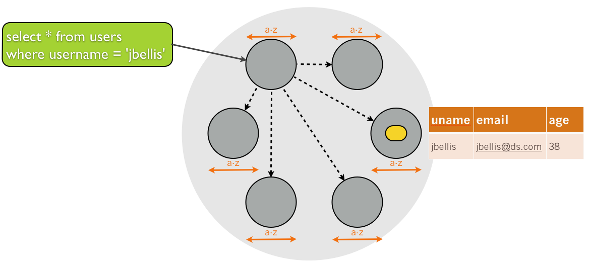
This causes index performance to scale poorly with cluster size: as the cluster grows, the overhead of coordinating the scatter/gather starts to dominate query performance.

Thus, for performance-critical queries the recommended approach has been to denormalize into another table, as Tyler outlined:

<pre>
CREATE TABLE users_by_name (
 username text PRIMARY KEY,
 id uuid
);
</pre>

Now we can look look up users with a partitioned primary key lookup against a single node, giving us performance identical to primary key queries against the base table itself--but these tables must be kept in sync with the&nbsp;users&nbsp;table by application code. &nbsp;

Materialized views give you the performance benefits of denormalization, but are automatically updated by Cassandra whenever the base table is:

<pre>
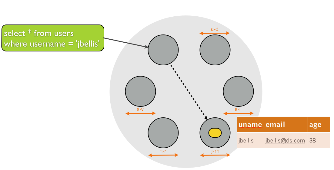
CREATE MATERIALIZED VIEW users_by_name AS 
SELECT * FROM users 
WHERE username IS NOT NULL
PRIMARY KEY (username, id);
</pre>

Now the view will be repartitioned by username, and just as with manually denormalized tables, our query only needs to access a single partition on a single machine since that is the only one that owns the j-m username range:
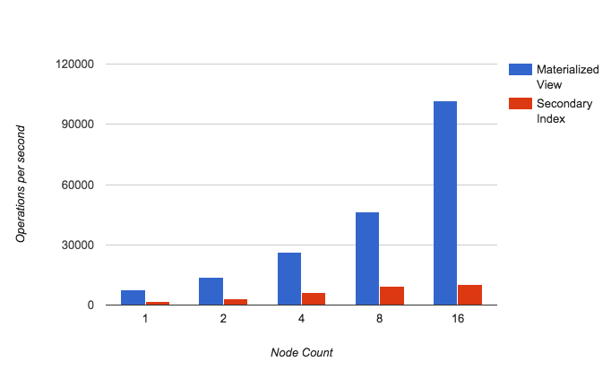
<img alt="Select User" data-align="center" data-entity-type="file" data-entity-uuid="78ae6e9d-e264-45d3-8284-dde7b935cb3b" src="https://www.datastax.com/sites/default/files/inline-images/Screen-Shot-2016-05-10-at-4.34.31-PM.png" />
The performance difference is dramatic even for small clusters, but even more important we see that indexed performance levels off when doubling from 8 to 16 nodes in the (AWS m3.xl) cluster, as the scatter/gather overhead starts to become significant:
<img alt="Operations per second and node count" data-align="center" data-entity-type="file" data-entity-uuid="a30d8064-d1dc-480c-ae31-a90e6d635739" src="https://www.datastax.com/sites/default/files/inline-images/pasted-image-0.png" />
<h2>Sidebar: When are Indexes Useful?</h2>

Indexes can still be useful when pushing analytical predicates down to the data nodes, since analytical queries tend to touch all or most nodes in the cluster anyway, making the primary advantage of materialized views irrelevant. &nbsp;

Indexes are also useful for full text search--another query type that often needs to touch many nodes--now that the&nbsp;<a href="http://rustyrazorblade.com/2016/02/cassandra-secondary-index-preview-1/">new SASI indexes</a>&nbsp;have been released.

<h2>Performance Impact of Materialized Views on Writes</h2>

What price do we pay at write time, to get this performance for reads against materialized views? &nbsp;

Recall that Cassandra&nbsp;<a href="http://docs.datastax.com/en//cassandra/2.2/cassandra/dml/dmlHowDataWritten.html">avoids reading existing values on UPDATE</a>. &nbsp;New values are appended to a commitlog and ultimately flushed to a new data file on disk, but old values are purged in bulk during&nbsp;<a href="http://docs.datastax.com/en/cassandra_win/2.2/cassandra/operations/opsConfigureCompaction.html">compaction</a>.

Materialized views change this equation. &nbsp;When an MV is added to a table, Cassandra is forced to read the existing value as part of the UPDATE. &nbsp;Suppose user jbellis wants to change his username to jellis:

<pre>
UPDATE users
SET username = 'jellis'
WHERE id = 'fcc1c301-9117-49d8-88f8-9df0cdeb4130';
</pre>

Cassandra needs to fetch the existing row identified by fcc1c301-9117-49d8-88f8-9df0cdeb4130 to see that the current username is jbellis, and remove the jbellis materialized view entry.

(Even for local indexes, Cassandra does not need to read-before-write. The difference is that MV denormalizes the entire row and not just the primary key, which makes reads more performant at the expense of needing to pay the entire consistency price at write time.)

Materialized views also introduce a per-replica overhead of tracking which MV updates have been applied.

Added together, here’s the performance impact we see adding materialized views to a table. &nbsp;As a rough rule of thumb, we lose about 10% performance per MV:
<img alt="Performance impact" data-align="center" data-entity-type="file" data-entity-uuid="f4b38189-1e9e-4eef-a2fe-f58b19014123" src="https://www.datastax.com/sites/default/files/inline-images/pasted-image-0-1.png" />
<h2>Materialized Views vs Manual Denormalization</h2>

Denormalization is necessary to scale reads, so the performance hits of read-before-write and batchlog are necessary whether via materialized view or application-maintained table. &nbsp;But can Cassandra beat manual denormalization?

We wrote a custom benchmarking tool to find out. &nbsp;<a href="https://github.com/tjake/mvbench">mvbench</a>&nbsp;compares the cost of maintaining four denormalizations for a playlist application for manual updates and MV.

Here’s what manual vs MV looks like in a 3 node, m4.xl ec2 cluster, RF=3, in an insert-only workload:
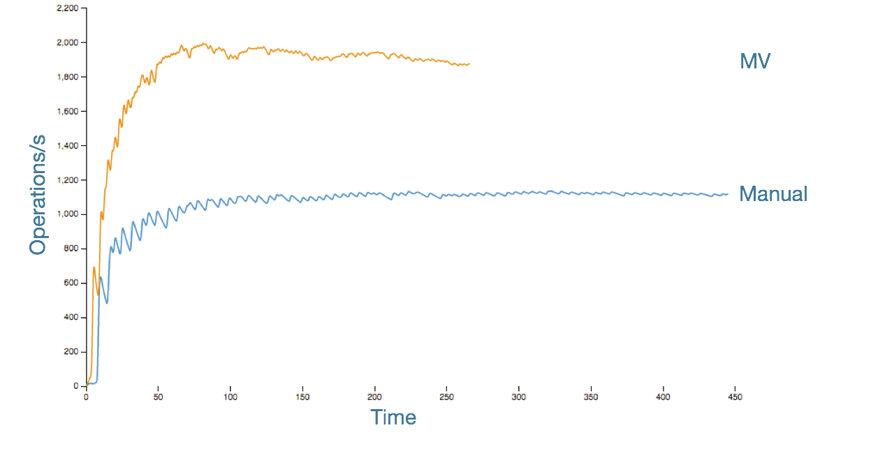
<img alt="Manual vs MV in 3 node cluster" data-align="center" data-entity-type="file" data-entity-uuid="4b26d8c0-9dda-4d3a-9bcc-9d7af874e59b" src="https://www.datastax.com/sites/default/files/inline-images/pasted-image-0-2.png" />
What we see is that after the initial JVM warmup, the manually denormalized insert (where we can “cheat” because we know from application logic that no prior values existed, so we can skip the read-before-write) hits a plateau and stays there. &nbsp;The MV, while faster on average, has performance that starts to decline from its initial peak.

To understand these results, we need to explain what the mvbench workload looks like. &nbsp;The data model is a table of playlists and four associated MV:

<pre>
CREATE TABLE user_playlists
(
 user_name text,
 playlist_name text,
 song_id text,
 added_time bigint,
 artist_name text,
 genre text,
 last_played bigint,
 PRIMARY KEY (user_name, playlist_name, song_id)
);
</pre>

The MV created are song_to_user, artist_to_user, genre_to_user, and recently_played. For the sake of brevity I will show only the last:

<pre>
CREATE MATERIALIZED VIEW IF NOT EXISTS mview.recently_played AS
 SELECT song_id, user_name
 FROM user_playlists
 WHERE song_id IS NOT NULL
 AND playlist_name IS NOT NULL
 AND user_name IS NOT NULL
 AND last_played IS NOT NULL
 PRIMARY KEY(user_name, last_played, playlist_name, song_id
);
</pre>

What is important to note here is that the base&nbsp;<tt>user_playlists</tt>&nbsp;table has a compound primary key. What is happening to cause the deteriorating MV performance over time is that our&nbsp;<a href="http://docs.datastax.com/en/cassandra/3.0/cassandra/operations/opsTuningBloomFilters.html">sstable-based bloom filter</a>, which is keyed by partition, stops being able to short circut the read-old-value part of the MV maintenance logic, and we have to perform the rest of the primary key lookup before inserting the new data.

<h2>MV Performance Summarized</h2>

As a general rule then, you can apply the following rules of thumb for MV performance:

<ul>
	<li>Reading from a normal table or MV has identical performance.</li>
	<li>Each MV will cost you about 10% performance at write time.</li>
	<li>For simple primary keys (tables with one row per partition), MV will be about twice as fast as manually denormalizing the same data.</li>
	<li>For compound primary keys, MV are still twice as fast for updates but manual denormalization can better optimize inserts. &nbsp;The crossover point where manual becomes faster is a few hundred rows per partition. &nbsp;<a href="https://issues.apache.org/jira/browse/CASSANDRA-9779">CASSANDRA-9779</a>&nbsp;is open to address this limitation.</li>
</ul>

Materialized View Performance in Cassandra 3.x

Jonathan EllisTechnology

Discover more

Share

More Technology

Getting Started with DataStax Astra DB and Amazon Bedrock

Why You Can't Miss Cassandra Summit

Mitigate the OpenAI Debacle with Open Source and Cloud

Supercharge AI Assistants with Superagent and DataStax

NoSQL and Vector DB
for Generative AI,
Instantly, At Scale