Sylvain Lebresne

<p>One of the change made in Apache Cassandra 3.0 is a relatively important <a href="https://issues.apache.org/jira/browse/CASSANDRA-8099">refactor of the storage engine</a>. I say refactor because the basics have not changed: data is still inserted in a memtable which get flushed over time to a sstable with compaction baby-sitting the set of sstables on disk, and reads uses both memtable and sstables to retrieve results. But the internal structure of the objects manipulated in those phases has changed, and that entails a significant amount of refactoring in the code. The principal motivation is that new storage engine more directly manipulate the structure that is exposed through CQL, and knowing that structure at the storage engine level has many advantages: some features are easier to add and the engine has more information to optimize.</p>

<h2>The old way</h2>

<p>Historically, the storage engine of Cassandra have been dealing with maps of (ordered) maps of binary data. That is, in memory, a table was represented by a Map&lt;byte[], SortedMap&lt;byte[], Cell&gt;&gt; (this is very much simplified but close enough from reality for the purpose of this post). The top-level keys of that map are the partition keys, and each partition (identified by its key) is a sorted key/value map. The inner values of that partition map is called a `Cell` mostly because it contains both a binary value and the timestamp that is used for conflict resolution (in practice, there is also different types of cells to deal with tombstones and counters, but that's outside the scope of this post). That legacy internal structure has the advantage of being very simple, and it was an almost direct match for the original API of Cassandra, the so-called Thrift API. The flip side however is that it is too simple. Real data almost always has more structure than that: it is often typed and you generally want something a bit more rich that just basic key/value. On the API side, this is why CQL has been introduced: it allows to express the structure/type of the data you store much more naturally, without requiring too much client side encoding. But internally, CQL has been so far still encoded on that relatively simple "map of map of binary data" storage engine. Which means that a lot of the structure the user provide through their CQL table definitions is encoded internally in a way that is largely opaque to the storage engine. For instance, a CQL row is internally represented by multiple "cells" and the storage engine has no real knowledge of how those cells related to each other. This is a problem for two main reasons:</p>

<ul>
	<li>some more advanced CQL features we want to add require some support from the storage engine, but that is much harder to do if you don't easy access to most of the basic structure.</li>
	<li>there is a lot of missed opportunity from a performance standpoint. Typically, the encoding of CQL over the legacy storage engine involves quite a few inefficiencies and duplication. As we'll see below, knowing about the full structure of the data in the storage engine avoids that duplication.</li>
</ul>

<h2>The new way</h2>

<p>So Cassandra 3.0 changes the internal structure of the objects manipulated by the storage structure and the basic idea is that it put that internal structure much closer to what CQL exposes. The old Map&lt;byte[], SortedMap&lt;byte[], Cell&gt;&gt; structure has been replaced by something that looks more like a Map&lt;byte[], SortedMap&lt;Clustering, Row&gt;&gt;. At the top-level, a table is still a map of partitions indexed by their partition key (which does mean partition keys composed of multiple CQL columns are still an encoding as far as the storage engine is concerned. This will likely change over time but isn't actually a big problem in practice). And the partition is still a sorted map, but it is one of rows indexed by their "clustering". The Clustering holds the values for the clustering columns of the CQL row it represents. And the Row object represents, well, a given CQL row, associating to each column their value and timestamp. I won't describe those objects in all their intricacies as this would be long and tedious. But this is open-source and interested parties are welcome to look for more details in the code. Starting, for instance, with the <a href="https://github.com/apache/cassandra/blob/trunk/src/java/org/apache/cassandra/db/Clustering.java">Clustering.java</a> and <a href="https://github.com/apache/cassandra/blob/trunk/src/java/org/apache/cassandra/db/rows/Row.java">Row.java</a> classes. Another aspect worth mentioning relates to deletions. Internally, Cassandra has the notion of Range Tombstones: a tombstone that cover a particular range within a partition. Before 3.0, because the storage engine has no real notion of a CQL row or a collection column (it only knows about cells, not how they relate to each other. It's the encoding of those cell that allows us to reconstruct how they relate), fairly common operations like a row deletion or a collection deletion (which also happens as part of inserting a new collection, as inserting a new collection require us to delete the previous) require a range tombstone. The problem is that by nature, because they cover ranges, these range tombstone are less efficient to deal with than simpler cell tombstones. In 3.0 however, as the storage engine knows about rows and collection, we're able to have specific row and collection tombstones. Those are more efficient that range tombstones, both in terms of the space we need to store them, but also in the amount of processing we need to handle them. Note that 3.0 still has range tombstones, which are still somewhat more costly that a simpler tombstone, but those are used much less frequently, only when you actually need to delete a range of rows, which is likely a lot less common (keeping in mind that deleting a full partition has also always been specialized and is fairly cheap). Another aspect that the refactor changed significantly is the sstable storage format.</p>

<h2>The storage format</h2>

<p>The storage format used for sstables is a (relatively simple) serialization of the internal data structure. The problem before 3.0 is that because a lot of the CQL structure is encoded on the internal structure, it is also opaque to the storage format. And that encoding is unfortunately not very efficient. In particular, each non-primary-key column of a CQL row is encoded by a different "cell", with both the column name and the full values of the clustering columns repeated every time. In practice, this means that if you do:</p>

<pre>
    CREATE TABLE events (
        id uuid,
        received_at timeuuid,
        property_1 int,
        property_2 text,
        property_3 float,
        PRIMARY KEY (id, received_at)
    );

    INSERT INTO events (id, received_at, property_1, property_2, property_3)
                VALUES (de305d54-75b4-431b-adb2-eb6b9e546014, now(), 42, 'foobar', 2.4);
</pre>

<p>then the resulting row will internally be comprised of 3 cells (for each "property" column) and each cell will be repeat 1) the received_at TimeUUID and 2) the actual column name. This is pretty wasteful and is one of the main reason why compression is enabled by default on SSTables: we need compression to reduce the cost of all that duplication. Still, compression is not perfect and having the repetition in the first place is not ideal. Further, compression has a CPU cost and we sometime would want to avoid compression without paying a huge cost in term of disk space. In C* 3.0 however, we don't have all those repetitions anymore since the full structure of CQL is preserved internally. The new storage format neither duplicate clustering values, nor write the full column name everywhere. These two changes offers offer great savings on disk, but the new file format also has a few additional trick up its sleeves (compared to the previous format at least):</p>

<ul>
	<li>the timestamps used for conflict resolution are delta-encoded and written using <a href="https://developers.google.com/protocol-buffers/docs/encoding?hl=en#varints">varints</a>. Further, they can sometimes be written only once for a given row when all the values in the row have the same timestamp. And as every value has an associated timestamp in Cassandra, this can provide a decent saving.</li>
	<li>the serialization of values is more type-aware. For instance, the storage format before 3.0 basically considered all values as blob and so a `bigint` value was actually taking 12 bytes: 8 bytes for the value plus 4 bytes to store the size of said value (even though it's always 8). That same value only take 8 bytes in 3.0.</li>
	<li>the new format also use varints every time we serialize a size. Typically, if you do store a blob value, it would be preceded on disk by 4 bytes for the size before 3.0, but in 3.0, if the blob is small, the value size itself might only take 1 or 2 bytes.</li>
</ul>

<p>All of these optimization conspire to a much more compact storage format. Consider for instance my example table events above, in which we insert a million rows (with a small text for <a>property_2</a>; see the <a href="https://gist.github.com/pcmanus/495d1d6f9418a99147ed">insertion script</a> for details). The size on disk resulting from that insertion is as follow: 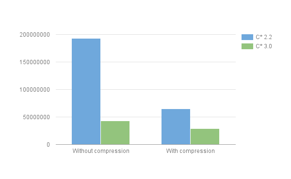<img alt="datasize_regular" src="https://www.datastax.com/sites/default/files/content/blog/datasize_regular.png" /> You can see that compression plays a very important to reduce the size in C* 2.2, but also that the size in C* 3.0 without compression is lower than the one on C* 2.2 with compression. And while compression still provides some benefits in 3.0, the difference is not as big, making the option of disabling compression a viable solution when you want lower latency and CPU usage. This is just one example however, and the exact savings will heavily depend on your schema and workload. Consider for instance the following (toy) table:</p>

<pre>
    CREATE TABLE smallsavings (
        k int PRIMARY KEY,
        v1 int,
        v2 text
    )
</pre>

<p>in which we insert a million rows with a fairly large string for v2 (of length 1000) every time (see the <a href="https://gist.github.com/pcmanus/db5adca5bcdd400d9f63">insertion script</a> for details). The results are the following ones 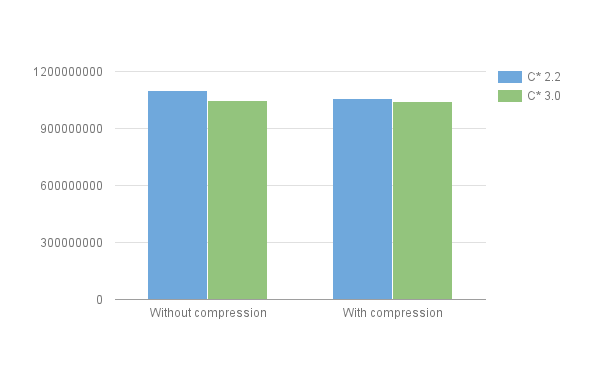<img alt="datasize_smallsavings" src="https://www.datastax.com/sites/default/files/content/blog/datasize_smallsavings.png" /> As can be seen, while C* 3.0 without compression is still more compact than C* 2.2 with compression, the difference is relatively small. This can be explained by 1) the fact that the table has no clustering and short column names and 2) the fact that the ratio of metadata to actual user data is lower due to the 1000 character string in all rows. On the other extreme, consider the following table:</p>

<pre>
    CREATE TABLE largesavings (
        k int,
        c text,
        my_first_value int,
        a_set_of_floats set,
        PRIMARY KEY (k, c)
    )
</pre>

<p>in which we insert a million rows with a fairly large string for c (of length 100) and a set of 50 floats in every row (see the <a href="https://gist.github.com/pcmanus/b731ba4278d4a6210589">insertion script</a> for details). The results are the following ones: <img alt="datasize_bigsavings" src="https://www.datastax.com/sites/default/files/content/blog/datasize_bigsavings.png" /> As you can see, the uncompressed 2.2 format is very inefficient, and even the uncompressed file in 3.0 is 2/3 of the compressed 2.2 version. This is due to a combination of factors:</p>

<ul>
	<li>the clustering value is somewhat large;</li>
	<li>the non primary key column names are also a tad long;</li>
	<li>we use a collection, which happens to multiply the effects of the 2 previous points.</li>
</ul>

<h2>A word on compact storage</h2>

<p>Tables using the COMPACT STORAGE exists mainly to expose table created in Thrift in CQL and it is discouraged to create new compact tables (as they have lots of limitations, and you're stuck with those limitations once you've signed up for COMPACT STORAGE). However, before 3.0, one could been tempted to create compact table due to the fact that the size on disk of a compact table was generally lower than the same table without COMPACT STORAGE. This is in fact the historic reason for the naming. But in 3.0, that advantage disappears. In fact a table will have the exact same internal layout whether is uses COMPACT STORAGE or not, so there will be no impact at all on the size on disk. Thankfully, it is not that the size used by compact tables is worth in C* 3.0, it is in fact better. Consider the results of inserting a million row to a simple table with and without compact storage in C* 2.2 and C* 3.0 (there is only one entry for 3.0 as, as we just said, using COMPACT STORAGE makes no difference whatsoever on the size on disk): 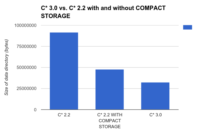<img alt="compact_storage_comparison" src="https://www.datastax.com/sites/default/files/content/blog/compact_storage_comparison.png" /> So, do not use COMPACT STORAGE on new tables. The option still exists only to allow thrift compatibility through restrictions on CQL functionality, but it has no effect on the actual bytes written to disk, nor to any processing done by the database (if anything, more work is done for compact storage table just to validate the restrictions applied to them).</p>


Build and scale cloud native apps

Discover the benefits of DBaaS and why your apps deserve an upgrade.

Learn about NoSQL Databases

Learn about NoSQL databases with Apache Cassandra and Astra DB.

2022 Recap: A Year for Customers, Community, and Real-Time Data

Highlights from 2022 and a glimpse into the year ahead.

ViewingTechnical How To’s

Putting some structure in the storage engine

Sign up for our Developer Newsletter