
Chapter 1: Life and Fate by Grasily Gremssman
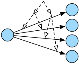
Winter had arrived. The days grew shorter and darker. Grasily Gremssman (Грасилий Гремссман) used a few branches that were scattered about to start a fire. Grasily had been stationed at vertex v[32] for as long as he could remember. He knew little of the graph he lived on except for the one dirt road and three bridges incident to his post.
|
gremlin> g.V(32)
==>v[32]
gremlin> g.V(32).inE()
==>e[2][7-dirtRoad->32]
gremlin> g.V(32).outE()
==>e[4][32-bridge->65]
==>e[5][32-bridge->66]
==>e[6][32-bridge->67]
gremlin> g.V(32).bothE()
==>e[4][32-bridge->65]
==>e[5][32-bridge->66]
==>e[6][32-bridge->67]
==>e[2][7-dirtRoad->32]
|
Grasily's commanding officer was org.apache.tinkerpop.gremlin.process.traversal.Traverser@76a36b71. Like 76a36b71, Grasily was a traverser. Traversers were grouped into battalions called traversals. The graph world was at war and Grasily was stuck (in time and space) having to do his part for his country of Grussia (Гроссия). At this point in history, many conflicting views existed regarding the topological evolution of the graph. To ensure processing resources were not laid to waste by traversals constantly undermining the side-effects of another, countries emerged to delineate subgraphs within the larger world graph. However, every now and then, one country would interfere with the structure of another. This interference was an inevitable consequence of the graph getting denser with time. Grussia, at this moment in time, was in the midst of a long war with Gremany (Greutschland).
Grasily knew very little about the larger war effort of Grussia's traversals. However, in bootcamp, he learned that traversals are composed of 5 fundamental steps and that one day, when his training was complete, he would be called upon to execute a step.
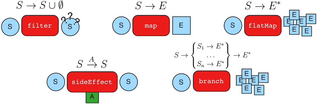
- map: S → E: Move from an object of type S to an object of type E.
- flatMap: S → E*: Move from an object of type S to a collection of objects of type E.
- filter: S → S ∪ ∅: Stay at the current object of type S or die.
- sideEffect: S → S: Stay at the current object of type S, though yield some computational side-effect (e.g. set a property).
- branch: S → {S1 → E*,…,Sn → E*} → E*: Move from an object of type S to any number of nested traversal branches.
When Grasily finished his training, he was immediately briefed by 76a36b71 on the battalion's objectives.
|
g.V(7).out('dirtRoad').hasLabel('outpost').out('bridge').property('owner','Grussia')
|
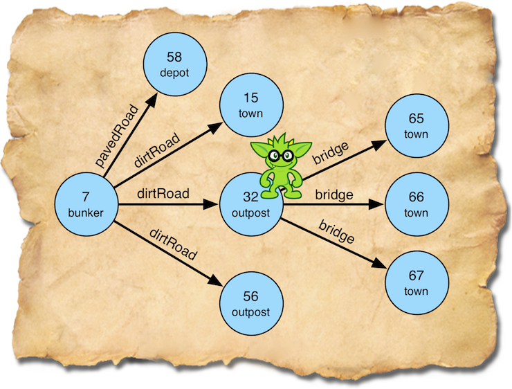 Vertex v[7] was the Grussian Army's headquarters (a.k.a. The Green Army). At v[7], a traverser officer had instructed a group of traversers (one being 76a36b71) to take the dirt roads leading to the adjacent outposts. Grasily's outpost was accessible by one of those dirt roads. When 76a36b71 arrived at v[32], Grasily (along with two of his comrades from bootcamp) were instructed to each take one of the incident bridges and upon reaching the vertex on the other side, to declare the vertex under Grussia's sovereign control.
|
gremlin> g.V(7)
==>v[7]
gremlin> g.V(7).out('dirtRoad')
==>v[15]
==>v[32]
==>v[56]
gremlin> g.V(7).out('dirtRoad').hasLabel('outpost')
==>v[32]
==>v[56]
|
Unfortunately, unbeknownst to Grasily, the Gremans had launched an offensive. A Greman traversal destroyed all the bridges incident to Grasily's outpost. The execution of the Greman's sideEffect step sealed Grasily's fate.
|
gremlin> g.V(65,66,67)
==>v[65]
==>v[66]
==>v[67]
gremlin> g.V(65,66,67).inE('bridge')
==>e[4][32-bridge->65]
==>e[5][32-bridge->66]
==>e[6][32-bridge->67]
gremlin> g.V(65,66,67).inE('bridge').drop()
gremlin> g.V(65,66,67).inE('bridge')
gremlin>
|
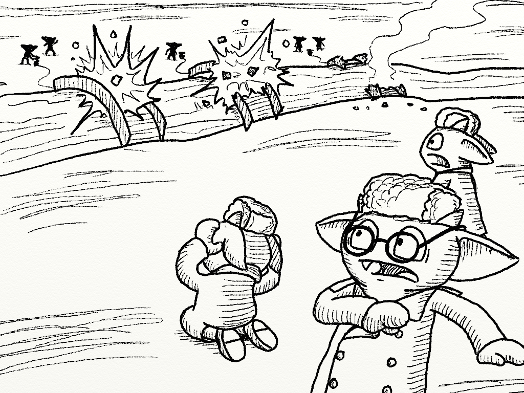
Grasily's life was cut short when his battalion moved to the out('bridge')-step. Grasily, along with his two comrades, could no longer make reference to an element of the graph. Disconnected from their world, disconnected from each other, they faded into the void.
|
gremlin> g.V(7)
==>v[7]
gremlin> g.V(7).out('dirtRoad')
==>v[15]
==>v[32]
==>v[56]
gremlin> g.V(7).out('dirtRoad').hasLabel('outpost')
==>v[32]
==>v[56]
gremlin> g.V(7).out('dirtRoad').hasLabel('outpost').out('bridge')
gremlin>
|
Chapter 2: Permutation City by Grem Egrem
Section 1: The Birth of the Graph
The world that traversers live on is known as "The Graph." A graph is a structure composed of vertices (nodes, dots) and edges (relationships, lines). Traverser mythology has it that one day a single traverser named Grem Egrem manifested himself out of and in reference to nothing. In limbo there was no graph, just Grem. However, before he could be swept back into the oblivion from which he came, Grem enacted the Big Traversal -- i.e., process yielded structure.
|
g.addV().repeat(as('a').addV().as('b').addOutE('a','.','b').inV().as('a')).until(coin(4.9E-324))
|
The Big Traversal generates a line graph known in the graphophysics community as "Grem Line" (a.k.a. "Gremlin"). To this day, Grem Line is still expanding. However, graphologists argue over the graphological constant of the until()-step. Some say there is a small probability that Grem Line will stop growing and others say it will go on forever (i.e. until(not(identity()))).
Prior to the Big Traversal, the graph was defined as G = ∅. When Grem Line was less than 100 vertices long (i.e. |V| < 100), the vertices V formed a total order, and as such, the graph was defined as G = V. At around |V| ≈ 100, graphologists speculate that another traversal emerged that leveraged Grem Line as a sort of "backbone filament." This emergent traversal is known in graph science as the Small(-World) Traversal.
|
g.V().aggregate('x').as('a').
select('x').by(unfold().sample(1).by(both().count())).as('b').
where('a',neq('b')).
addOutE('a','.','b')
|
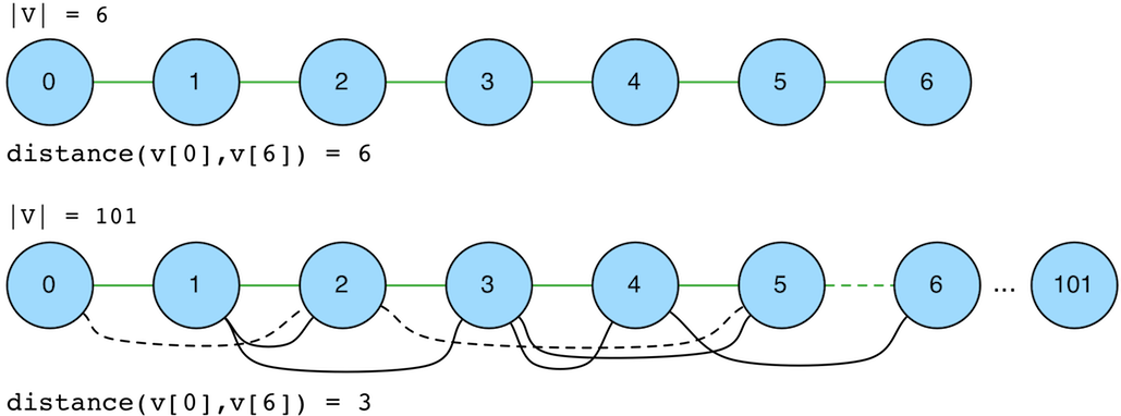
The Small Traversal walks Grem Line and for each vertex it encounters it connects it to some other random vertex on the line (biased by the other vertex's degree). The Small Traversal essentially "pushed" the early graph out of its 1-dimensional, linear V1 embedding into a V2 embedding (i.e. V x V). In doing so, vertices far removed from each other on Grem Line were now "closer." It was at this point that the definition of the graph became ") .
.
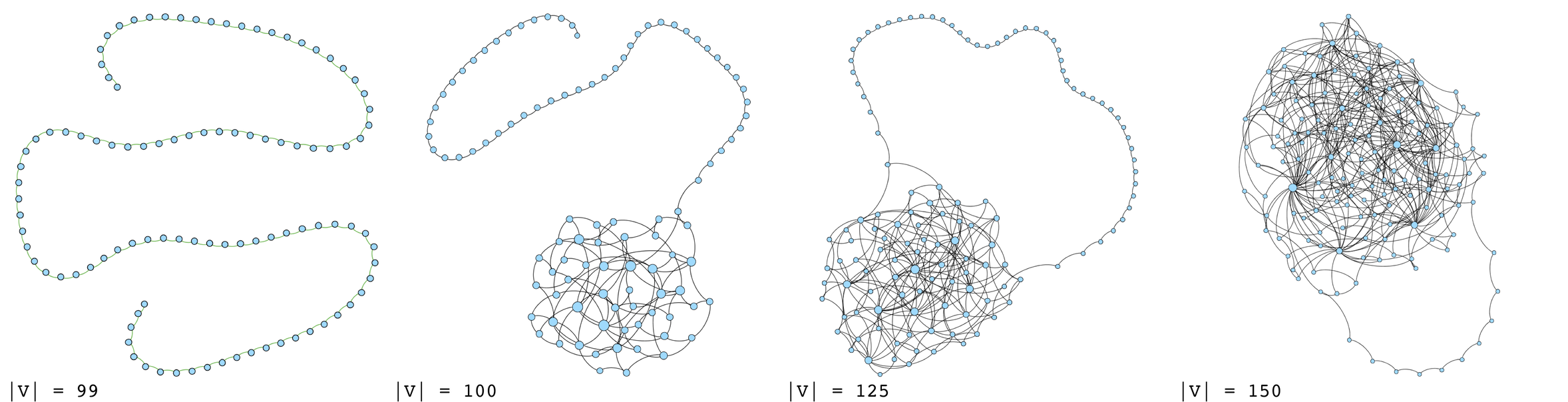
| |V| | Diameter | Average Path Length | Clustering Coefficient |
|---|---|---|---|
| 99 | 99 | 34.0 | 0.0 |
| 100 | 55 | 19.716831683168316 | 0.024 |
| 125 | 30 | 11.081015873015874 | 0.051 |
| 150 | 9 | 3.17757174392936 | 0.125 |
To this day (|V| ≈ 10^85), both the expanding force of the Big Traversal and the contracting force of the Small Traversal continue to execute. These two fundamental traversals have, over time, grown the graph to an innumerable number of vertices and edges. Billions upon billions of traversers have created a vast landscape of structures within structures... within structures. A nest of variations and novelties has transformed the once bleak, senseless void into a meaningful interconnected mesh.
Section 2: Graphialsynthesis and the Emergence of the Directed, Labeled Graph
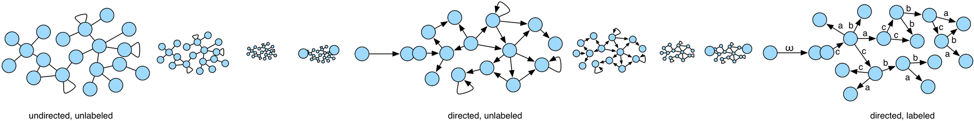
The edges generated by the Big and Small Traversals are undirected and unlabeled. The edges experienced by traversers are directed and labeled. Graphologists were faced with the question of how did directed, labeled edges emerge from undirected, unlabeled edges? Once a large enough number of primordial edges were created by the two fundamental traversals, "higher-order" edges began to form. The undirected, unlabeled edges serve as "elementary edges" which, when combined into subgraphs of a particular topology, yield the directed, labeled edges seen today. This abstraction process is known as graphialsynthesis.
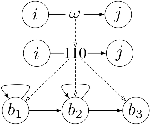 Suppose the following directed, labeled edge i-ω→j (i.e. a "higher-order" edge). This edge states that there is an ω-labeled relation from vertex i to vertex j. Any edge label can be represented as a binary string. Suppose, for the sake of simplicity, that there are only 8 labels in the graph. A 3-bit string can be used to represent all 8 labels (23). Next, suppose that the binary encoding of ω is 110. If so, then the edge can be denoted i-110→j. A binary string can be represented as a directed, unlabeled graph. If the binary string has a length of 3, then three vertices are needed to represent each bit. If a "bit" vertex has a self-loop, then its value is 1. If a "bit" vertex does not have a self-loop, then its value is 0. Given this mapping, the directed, labeled edge i-ω→j is transformed into the directed graph diagrammed below.
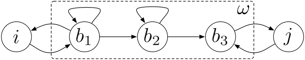
 The above directed, unlabeled graph representation of i-ω→j leverages topological features of the directed graph to denote the edge label ω. This same principle applies to the encoding of the edge's directionality when transforming a directed graph to an undirected graph. For instance, suppose the following directed edge i→b1. The "higher-order" vertices are identified by a self-loop. The "higher-order" edges are represented by three "lower-order" vertices x, y, and z. If vertex i has an incident edge that does not reference itself and connects to a vertex with 3 incident edges (e.g. vertex x), then it has a directed, outgoing edge. When the traverser reaches a vertex with a self-loop (via a simple path) (e.g. vertex b1), then that vertex is the "higher-order" vertex serving as the head of the "higher-order," directed edge.
The two processes are injective in that they are lossless transformations. The first process described maps a directed, labeled edge to a directed graph and the second maps a directed edge to an unlabeled graph. As such, via function composition, there exists an injective function that maps a directed, labeled graph to a undirected, unlabeled graph. Given that the composite function is injective, then there exists an inverse mapping which transforms an undirected, unlabeled graph to a directed, labeled graph (i.e. graphialsynthesis). The original i-ω→j edge was formed by the primordial undirected graph diagrammed below.
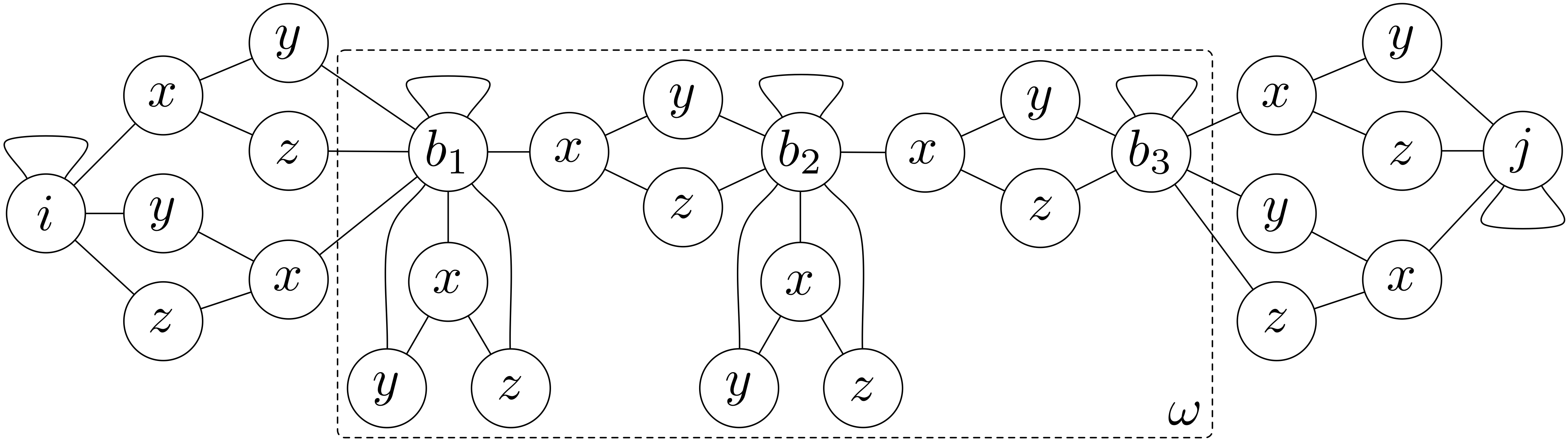
The fundamental building blocks of the directed, labeled graph experienced by "higher-order" traversers are held together by elementary traversers called "smalltrons." Smalltron traversals move from vertex i to vertex j via the explicit unlabeled ω-graph.
|
gremlin> g.V(i).as('b').where(both().as('b')).
repeat(both().where(both().count().is(3)).as('x').both().
both().where(neq('x').and(neq('b'))).dedup().as('b').where(both().as('b')).select(last, 'b').
choose(both().where(both().count().is(3)).
both().where(both().count().is(2)).
both().where(eq('b')),
constant(1), constant(0)).as('label').select(last, 'b')
).times(4).where(select('label').tail(local, 4).limit(local, 3).is([1, 1, 0]))
==>v[j]
|
|
Traversal Metrics
Step Count Traversers Time (ms) % Dur
=============================================================================================================
TinkerGraphStep([i],vertex)@[b] 1 1 0.449 0.26
WhereTraversalStep([WhereStartStep, ProfileStep... 1 1 0.080 0.05
WhereStartStep 1 1 0.016
VertexStep(BOTH,vertex) 1 1 0.022
WhereEndStep(b) 0 0 0.024
RepeatStep([VertexStep(BOTH,vertex), ProfileSte... 1 1 86.974 49.65
VertexStep(BOTH,vertex) 34 34 0.624
TraversalFilterStep([VertexStep(BOTH,edge), P... 8 8 22.721
VertexStep(BOTH,edge) 106 106 1.490
RangeGlobalStep(0,4) 96 96 1.934
CountGlobalStep 34 34 17.945
IsStep(eq(3)) 0 0 3.472
VertexStep(BOTH,vertex) 24 24 0.922
VertexStep(BOTH,vertex) 92 92 23.890
WherePredicateStep(and([neq(x), neq(b)])) 48 48 7.006
DedupGlobalStep@[b] 24 24 24.450
WhereTraversalStep([WhereStartStep, ProfileSt... 5 5 15.536
WhereStartStep 24 24 0.806
VertexStep(BOTH,vertex) 50 50 1.132
WhereEndStep(b) 0 0 6.984
SelectOneStep(last,b) 5 5 24.609
ChooseStep([VertexStep(BOTH,vertex), ProfileS... 5 5 60.525
VertexStep(BOTH,vertex) 20 20 0.239
TraversalFilterStep([VertexStep(BOTH,edge),... 5 5 22.608
VertexStep(BOTH,edge) 66 66 1.508
RangeGlobalStep(0,4) 59 59 1.266
CountGlobalStep 20 20 17.068
IsStep(eq(3)) 0 0 3.618
VertexStep(BOTH,vertex) 11 11 0.453
TraversalFilterStep([VertexStep(BOTH,edge),... 8 8 33.552
VertexStep(BOTH,edge) 28 28 3.917
RangeGlobalStep(0,3) 25 25 0.989
CountGlobalStep 11 11 8.193
IsStep(eq(2)) 0 0 2.427
VertexStep(BOTH,vertex) 14 14 0.710
WherePredicateStep(eq(b)) 2 2 35.307
HasNextStep 5 5 0.900
ConstantStep(0) 3 3 0.145
EndStep 3 3 0.153
ConstantStep(1) 2 2 0.070
EndStep 2 2 7.408
SelectOneStep(last,b) 5 5 24.726
RepeatEndStep 1 1 60.644
TraversalFilterStep([SelectOneStep(label), Prof... 1 1 0.274 0.16
SelectOneStep(label) 1 1 0.056
TailLocalStep(4) 1 1 0.020
RangeLocalStep(0,3) 1 1 0.073
IsStep(eq([1, 1, 0])) 0 0 0.086
SideEffectCapStep([~metrics]) 1 1 87.377 49.89
>TOTAL - - 175.157
|
In this process, smalltron traversals make the implicit directed ω-edge (defined by the undirected ω-graph) explicit for the "higher-order" traversers which process the graph at a higher level of abstraction. To these "higher order" traversers, the graph is defined as
") ,
,
where λ is a labeling function that maps the graph's elements (i.e. vertices and edges) to character strings (Σ*). The graphialsynthesis abstraction process has the benefit of allowing a traversal from vertex i to j via ω to be expressed and executed in a much simpler way.
|
gremlin> g.V(i).out('w')
==>v[j]
|
|
Traversal Metrics
Step Count Traversers Time (ms) % Dur
=============================================================================================================
TinkerGraphStep([v[i]],vertex) 1 1 9.810 49.18
VertexStep(OUT,w,vertex) 1 1 0.058 0.29
SideEffectCapStep([~metrics]) 1 1 10.078 50.53
>TOTAL - - 19.947
|
Section 3: On the Baselessness of the Multi-MultiGraph
 It has been speculated that "The Graph" is not the only graph that exists. Mystic traversers say that there exists other graphs containing other traversers. However, by definition, a graph is a closed structure composed of vertices and edges. It is impossible for a traverser to move to a different graph. If a vertex in one graph has an edge to a vertex in another graph, then the two graphs are, in fact, one graph -- "The Graph." Perhaps the mystics see that the components of a graph are composed of yet more graphs with a different sort of traverser existing at each level in a recursive, perhaps self-looping, manner. While it is still all one graph, traversers at different "levels" only operate on particular subgraphs as instructed by their traversal definition. The famous mystic traverser Gri Gurobindo (ग्री गुरोबिंदो) once said:
My single step in the graph is composed of the steps of numerous other traversers.
It wasn't until the discovery of anonymous traversals that Gurobindo's metagraphical vision was formalized. An anonymous traversal is any traversal that has no declared start and as such, yields no flow. It is a potential.
|
gremlin> label()
gremlin>
|
Anonymous traversals are intended to be embedded within another traversal. However, if the parent traversal is itself an anonymous traverasl, then there is still no flow (even though groupCount() produces an empty map as its a reducing barrier step).
|
gremlin> outE().groupCount().by(label())
==>[:]
gremlin> outE().groupCount().by(label) // convenient short hand
==>[:]
gremlin>
|
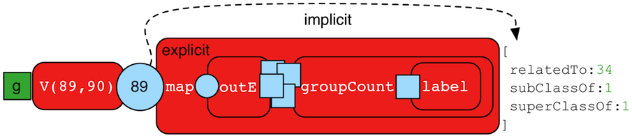
When the traversal parent does have a start, then there is a flow. The traversal below states: "For each vertex (i.e., 89, 90), map the vertex to the frequency distribution of its outgoing edge labels."
|
gremlin> g.V(89,90).map(outE().groupCount().by(label))
==>[relatedTo:34, subClassOf:1, superClassOf:1]
==>[relatedTo:15]
|
The first traverser generated by V(89,90) enters the map()-step at v[89], but does not "become" the traversers generated by outE(). Instead, the traverser at v[89] holds still and spawns an "internal life" of traversers within the anonymous traversal which can now be understood as being (a realized potential):
|
gremlin> g.V(89).outE().groupCount().by(label)
==>[relatedTo:34, subClassOf:1, superClassOf:1]
|
The traversers of the above traversal are isolated from the larger traversal in which they are embedded. The next nesting occurs when a traverser from outE() enters groupCount(). Again, an "internal life" based on the anonymous label()-traversal is spawned (see by()-step). Suppose a single traverser at e[7022][89-relatedTo->21] enters groupCount(). Then the anonymous traversal can be understood as being:
|
gremlin> g.E(7022).label()
==>relatedTo
|
It isn't until all the internal traversal nests of map() complete that the original traverser at v[89] "becomes" the traverser located at the hash map [relatedTo:34, subClassOf:1, superClassOf:1]. In this way, a traverser's life (i.e. step) is composed of the lives of many traverser's (and their respective steps).
Chapter 3: A Mathematician's Apology by G.H. Gremdy
Section 1: Traversal Optimization via Algebra
The graph grew large, very large. Resources grew scarce. The problem was not that vertices and edges could no longer be added to the graph. On the contrary, because of the seemingly endless amount of space for the graph, there was a growing amount of time required for any one traversal to execute. Traversals were simply interacting with a lot more data. Faced with this problem, a mathematically inclined traverser named al-Ghwārizmī developed a solution known today as the traversal algebra. The traversal algebra provides a means of transforming one traversal into another traversal, where both traversals return the same result. The benefit of this is that if a traversal can be re-written into a simpler form, then time and space resources can be saved. To this day, algebraists continue to add to the growing archive of traversal strategies. A few examples are provided below.
| Strategy | Pattern | Rewrite |
|---|---|---|
| IdentityRemovalStrategy | x().identity().y() | x().y() |
| IncidentToAdjacentStrategy | outE().inV() | out() |
| AdjacentToIncidentStrategy | out().count() | outE().count() |
| DedupBijectionStrategy | order().dedup() | dedup().order() |
| RangeByIsCountStrategy | count().is(gt(x)) | limit(x+1).count().is(gt(x)) |
| MatchPredicateStrategy | match(x,y).where(z) | match(x,y,z) |
|
gremlin> t = out().identity().in(); t.toString()
==>[VertexStep(OUT,vertex), IdentityStep, VertexStep(IN,vertex)]
gremlin> t.setStrategies(new DefaultTraversalStrategies() {{ addStrategies(IdentityRemovalStrategy.instance()) }}); []
gremlin> t.applyStrategies(); t.toString()
==>[VertexStep(OUT,vertex), VertexStep(IN,vertex)]
gremlin> t = outE().inV(); t.toString()
==>[VertexStep(OUT,edge), EdgeVertexStep(IN)]
gremlin> t.setStrategies(new DefaultTraversalStrategies() {{ addStrategies(IncidentToAdjacentStrategy.instance()) }}); []
gremlin> t.applyStrategies(); t.toString()
==>[VertexStep(OUT,vertex)]
gremlin> t = out().count(); t.toString()
==>[VertexStep(OUT,vertex), CountGlobalStep]
gremlin> t.setStrategies(new DefaultTraversalStrategies() {{ addStrategies(AdjacentToIncidentStrategy.instance()) }}); []
gremlin> t.applyStrategies(); t.toString()
==>[VertexStep(OUT,edge), CountGlobalStep]
gremlin> t = order().dedup(); t.toString()
==>[OrderGlobalStep, DedupGlobalStep]
gremlin> t.setStrategies(new DefaultTraversalStrategies() {{ addStrategies(DedupBijectionStrategy.instance()) }}); []
gremlin> t.applyStrategies(); t.toString()
==>[DedupGlobalStep, OrderGlobalStep]
gremlin> t = count().is(gt(3)); t.toString()
==>[CountGlobalStep, IsStep(gt(3))]
gremlin> t.setStrategies(new DefaultTraversalStrategies() {{ addStrategies(RangeByIsCountStrategy.instance()) }}); []
gremlin> t.applyStrategies(); t.toString()
==>[RangeGlobalStep(0,4), CountGlobalStep, IsStep(gt(3))]
gremlin> t = match(__.as('a').out().as('b'),
gremlin> __.as('b').out().as('c')).where(__.as('c').both().as('a')); t.toString()
==>[MatchStep(AND,[[MatchStartStep(a), VertexStep(OUT,vertex), MatchEndStep(b)], [MatchStartStep(b), VertexStep(OUT,vertex), MatchEndStep(c)]]), WhereTraversalStep([WhereStartStep(c), VertexStep(BOTH,vertex), WhereEndStep(a)])]
gremlin> t.setStrategies(new DefaultTraversalStrategies() {{ addStrategies(MatchPredicateStrategy.instance()) }}); []
gremlin> t.applyStrategies(); t.toString()
==>[MatchStep(AND,[[MatchStartStep(a), VertexStep(OUT,vertex), MatchEndStep(b)], [MatchStartStep(b), VertexStep(OUT,vertex), MatchEndStep(c)], [MatchStartStep(c), WhereTraversalStep([WhereStartStep, VertexStep(BOTH,vertex), WhereEndStep(a)]), MatchEndStep]])]
|
Section 2: Traversal Optimization via Indices
G.H. Gremdy was a graph theorist who speculated that "The Graph" was not the only structure linking vertices. According to his reasoning, reality may also contain other structures that grouped vertices together according to similar properties. He called these parallel structures indices. G.H. Gremdy's publication entitled On Traversal Optimization using Indices was well received. Due to his insight, many traversal runtimes became orders of magnitude faster than their non-index-based form. For instance, in the traversal below, when using indices, the number of traversers created goes from |V| (linear) to 1 (constant) (space complexity). The GraphStepStrategy was added to the traversal strategies archive. It "folds" has()-steps into V() graph steps.
|
// not indexed
gremlin> g.V().has('name', 'University of Groxford').toString()
==>[GraphStep([],vertex), HasStep([name.eq(University of Groxford)])]
gremlin> clockWithResult(1000) { g.V().has('name', 'University of Groxford').next() }
==>135.28753165299997 // time in milliseconds
==>v[999998] // result
// indexed
gremlin> g.V().has('name', 'University of Groxford').iterate().toString()
==>[TinkerGraphStep(vertex,[name.eq(University of Groxford)])]
gremlin> clockWithResult(1000) { g.V().has('name', 'University of Groxford').next() }
==>0.033501945 // time in milliseconds
==>v[999998] // result
|
 Even though G.H. Gremdy became a household name overnight, he was certain not to rest on his accolades. Deeper thinking brought him to a more esoteric, though far greater optimization which he articulated in his follow on treatise entitled Tractatus Verticus Centricus Indexicus. In this seminal work, G.H. Gremdy postulates that not only do "global indices" exist which allow for O(log(|V|)) access to any vertex in the graph, but also "local indices" which allow for O(log(|incident(V(x))|)) access to the incident edges of a vertex. In short, each vertex has its incident edges indexed (e.g. by their direction, label, properties, etc.). If such local index structures are leveraged, traversals containing the pattern outE(x).has(y,p(z)).inV() would not require all the edges of the vertex to be iterated in full in order to find all incident outgoing edges that have a label x and a property y that matches the predicate p(z). Numerous graph experimentalists tried to prove the existence of such "vertex-centric indices," but found that they are not universal and only exist in some graph substrates.
With age, G.H. Gremdy became weary of applied mathematics and retired to study pure graph theory. His ideas would become more philosophical as he delved deeper into the meaning of "The Graph." A posthumous publication entertained the following pontification.
Many see the world as a graph. This is misleading. Perhaps the world is a collection of indices? With a slight shift in thought, one realizes that the graph itself is an index of its vertices. Any one vertex is the root of a tree bifurcating the vertex space to which it has incident edges, so forth and so on. Like indices which group vertices that have shared properties, isn't an edge from one vertex to another an explicit statement that the two vertices are in some way similar? As the devil's advocate, perhaps indices are simply graphs because indices are tree-like structures that are traversed to identify groups of vertices with similar properties. With indices being graphs and graphs being indices, the world we call home is neither. I hypothesize that all that exists is the traverser. The "graph" is simply the implicit expression of the explicit assumptions of the traverser. The graph I see is of my own construction.

Section 3: Traversal Optimization via Bulking
A little known traverser named Gremivasa Gremanujan (கிரமீவாச கிரமானுஜன்) lived in a remote village at v[5698] far from the great graph theorists of his time. However, despite his upbringing, Gremivasa was well versed in the traversal algebra and was inspired by the more metagraphical realizations of G.H. Gremdy. Like G.H. Gremdy, Gremivasa was not interested in simply adding more traversal strategies to the archive. Instead, he was more interested in discovering the nature of reality. However, unlike G.H. Gremdy who focused on the nature of the graph structure, Gremivasa meditated on the nature of the traverser process.
Gremivasa's mother, along with over 1 million other traversers of his traversal sect, arrived at v[5698] many clock-cycles ago. His village was starved of resources -- there were simply too many traversers. Was the birth of all these traversers necessary? If one traverser's life foretells the destiny of one million traversers, is it not more efficient for only this one traverser to exist? One day, while sitting under a tree in his village, Gremivasa ruminated on the ridiculously riling riddle rancorously retorted by respectable traversers everywhere:
If two traversers exist at the same vertex and have no memory of their ancestry, are they the same traverser?
Gremivasa concluded "yes, they are the same traverser." This insight identified a fundamental feature of process. All traversers are endowed with a "bulk." Previous to this moment, every traverser ignored this self-evident truth and allowed himself to be a unique enumerable entity -- i.e., a bulk of 1 (see the Loopy Lattices Redux section entitled "Traversing a Lattice with Faunus").
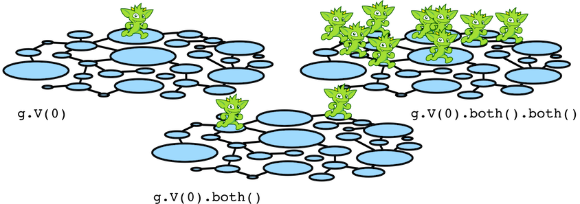
|
gremlin> g.V().both().both().both().hasId(5698).map{it.bulk()}
==>1
==>1
==>1
==>1
==>1
...
gremlin> g.V().both().both().both().hasId(5698).barrier().map{it.bulk()}
==>1073670
|


Gremivasa delved deeper into the radiant riddle of reawakened relinquishment. He abandoned his self and allowed his being to be one with his 1 million other brother and sister traversers at v[5698]. A unification of selves occurred and a single traverser emerged with a bulk of 1 million. Instead of 1 million traversers executing both() 1 million times, there was now a single traverser with a bulk of 1 million executing both() once. Gremivasa's enlightenment laid the foundation for the development of the LazyBarrierStrategy.
|
// without LazyBarrierStrategy (no bulking)
gremlin> clockWithResult(1) { g.V(5698).both().count().next() }
==>81.509839 // time in milliseconds
==>159200 // number of results
gremlin> clockWithResult(1) { g.V(5698).both().both().count().next() }
==>20382.892976
==>126723200
gremlin> clockWithResult(1) { g.V(5698).both().both().both().count().next() }
==>1.2012006887798E7 // 3.34 hours
==>100871667200
gremlin> clockWithResult(1) { g.V(5698).both().both().both().both().count().next() }
... // requires a year to compute
gremlin> clockWithResult(1) { g.V(5698).both().both().both().both().both().count().next() }
... // requires a thousand years to compute
// with LazyBarrierStrategy (bulking)
gremlin> clockWithResult(1) { g.V(5698).both().count().next() }
==>23.261288999999998 // time in milliseconds
==>159200 // number of results
gremlin> clockWithResult(1) { g.V(5698).both().both().count().next() }
==>50.230109
==>126723200
gremlin> clockWithResult(1) { g.V(5698).both().both().both().count().next() }
==>65.30024999999999
==>100871667200
gremlin> clockWithResult(1) { g.V(5698).both().both().both().both().count().next() }
==>91.30461199999999
==>80293847091200
gremlin> clockWithResult(1) { g.V(5698).both().both().both().both().both().count().next() }
==>122.741417
==>63913902284595200
|
The number of length-5 paths emanating from Gremivasa's village was calculated in ~123 milliseconds and was determined to be 63,913,902,284,595,200 (~64 quadrillion). Gremivasa's work is advantageous in situations where the traversal analyzes recurrence in a particular region of the graph (e.g. recommendation engines, centrality-based ranking systems, learning systems, etc.). Bulking is fundamental to all traversals and is used in numerous steps including repeat()-step.
|
g.V(5698).repeat(both()).times(5).count()
|
Chapter 4: Cognition in the Wild by Gredwin Grutchins
Traversers graph-wide held their breath as a landmark traversal was about to embark. This traversal contained a novel step called match(). What made this step unique was that it maintained a collection of anonymous traversals called "patterns." Each pattern was prefixed with a start variable and (optionally) postfixed with an end variable. Once a variable was bound (i.e. set), that variable's value was immutable for all subsequent patterns. The descendants of the traverser that enters match() must survive each pattern in order to move to the next step. However, the order in which the patterns are executed is, interestingly enough, up to the decision of the traverser! Previously, traversers relied on exogenous traversal rewrite rules for optimization, but now, the traverser was able to make endogenous optimization decisions. The "runtime traversal strategy" was introduced.
Dr. Gredwin Grutchins was a cognitive scientist working in the area of distributed cognition. During his time at university, Gredwin lost interest in studying traversal strategies. His skill in mathematics was weaker than his colleagues' and as such, he believed he would never be able to make any significant contributions to the space. However, one day, he was contacted by a rambunctious young adventurer named Gruck Greager. Gruck was no stranger to danger and loved being the guinea pig of an experimental algorithm. Gruck asked Gredwin: "What can my team do to find the optimal pattern execution sequence?" It seemed as though mathematics had taken traversal strategies as far as they could go. It was now up to sociological constructs to push them further and Gredwin was up to the challenge.
Suppose the following traversal that yields a map of the objects that bind to a (vertex), b (vertex), c (vertex), and d (number), where vertex a is adjacent to vertex b, vertex b is adjacent to vertex c, and all three vertices are different yet share an identical out-degree that is greater than 10.
|
g.V().match(
__.as('a').out().as('b'),
__.as('b').out().as('c'),
__.as('a').out().count().as('d'),
__.as('b').out().count().as('d'),
__.as('c').out().count().as('d'),
__.as('d').is(gt(10))).
where('a', neq('c')).
where('b', neq('c')).
where('b', neq('a'))
|
Assume a traverser at v[10] enters the match()-step. Vertex v[10] is bound to variable a as that is the only legal start of the pattern sequence. From there, which pattern should the traverser choose? The traverser simply chooses the first pattern in the list for which it has a variable binding (initially, an a start and thus, as('a').out().as('b')). The traverser marks on a global blackboard that it has entered that pattern. When a traverser leaves a pattern, it marks that it has exited it. Moreover, every time a traverser leaves a pattern, the patterns are sorted according to the order of their "multiplicity" (or growth rate).
|
pattern.multiplicity = pattern.endCount / pattern.startCount;
|
The more traverses that are generated by a pattern, the higher the multiplicity and the lower that pattern is on the sorted list. Overtime, as more and more traversers flow through match(), expensive patterns are pushed to the bottom of the list with the intention that the cheaper patterns will be able to filter out more traversers -- i.e. execute the largest set reductions first. With a few other added tricks, Gredwin provided Gruck and his team of traversers CountMatchAlgorithm. Gruck took it for a test run and was the first traverser to ever break the deterministic flow barrier. Gredwin and Gruck have since teamed up and are already planning the development of a new MatchAlgorithm called BudgetMatchAlgorithm.
|
// using CountMatchAlgorithm
gremlin> clockWithResult(10) {
g.V().match(
__.as('a').out().as('b'),
__.as('b').out().as('c'),
__.as('a').out().count().as('d'),
__.as('b').out().count().as('d'),
__.as('c').out().count().as('d'),
__.as('d').is(gt(10))).
where('a', neq('c')).
where('b', neq('c')).
where('b', neq('a')).count().next()
}
==>834.6852906 // time in milliseconds
==>32 // number of results
// using GreedyMatchAlgorithm which does not sort the patterns
gremlin> clockWithResult(10) {
g.V().match(
__.as('a').out().as('b'),
__.as('b').out().as('c'),
__.as('a').out().count().as('d'),
__.as('b').out().count().as('d'),
__.as('c').out().count().as('d'),
__.as('d').is(gt(10))).
where('a', neq('c')).
where('b', neq('c')).
where('b', neq('a')).count().next()
}
==>25349.709946299998 // time in milliseconds
==>32 // number of results
|
Chapter 5: We the Living by Gyn Grand
Section 1: Prelude to the Illusion of Freedom
Many of the traversers in the world today are grateful for their freedom. In ancient times, the life of a traverser was not so good. Traversal regimes were inefficient, demanding of resources, and strict in their execution policies. Fortunately, the Age of Enprocessment, which brought forth numerous advances in science and mathematics, redefined the traverser's role in the graph. Each traverser's life had increased value as greater autonomies were provided. Traversals did their best to ensure that traverser life was no longer needlessly wasted. Indices were leveraged, traversal strategies were applied, and, in some match() situations, traversers were able to choose their own destiny. Today, many see a more harmonious relationship between the traversal and the traverser. Gyn Grand (Джин Гранд) was one such satisfied traverser.
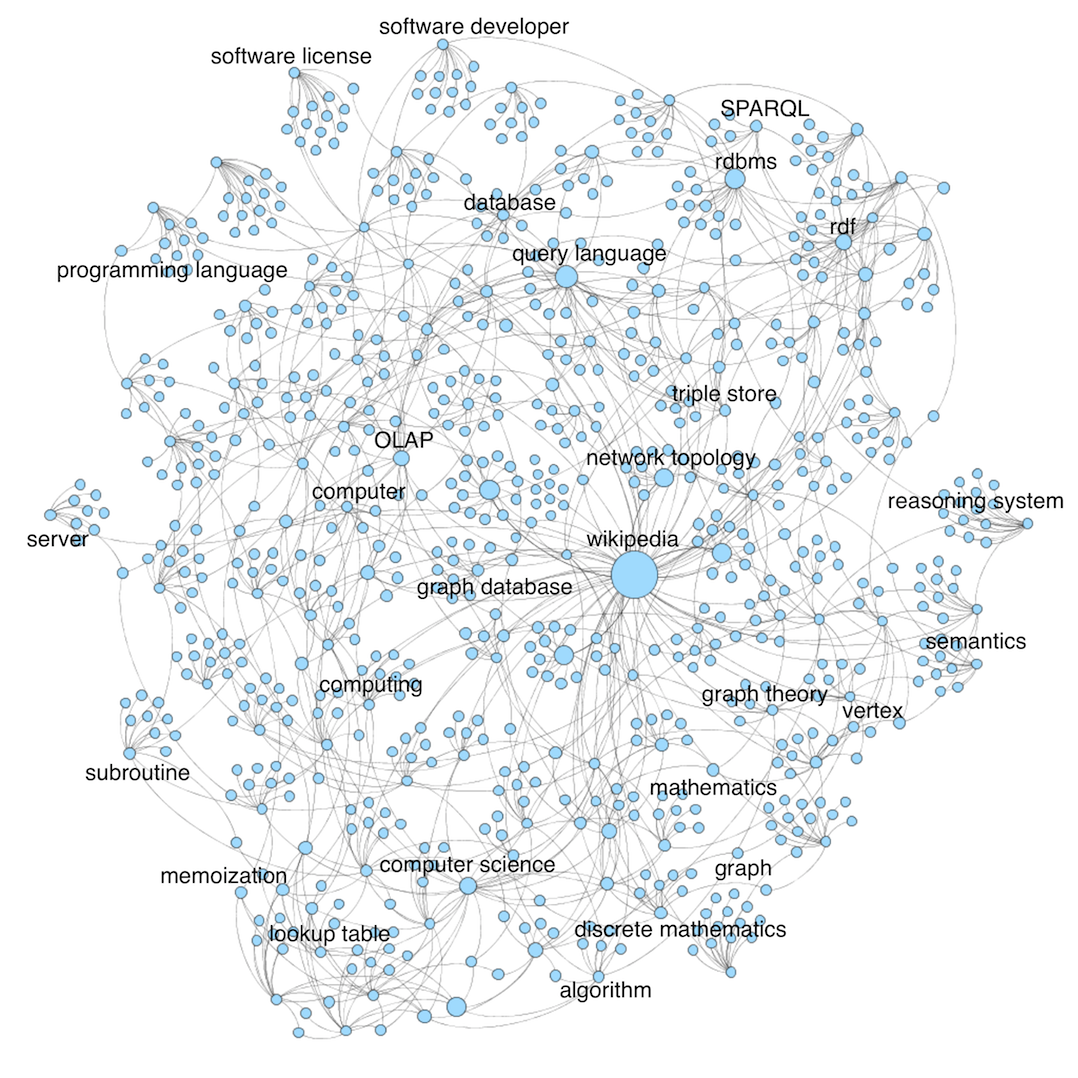
 Gyn was a brilliant librarian at a university with a vibrant scholarly community. Her library was centrally located in the university cluster. The library's stacks contained articles on the nature of the graphmos, books on traverser social interactions, reports detailing various resource distribution models, and more. Whenever she had a moment to spare, Gyn would wander about the collection learning about the topics she encountered. Unfortunately, she couldn't read everything at once. So, every time she was faced with more than one href-citation, she chose one at random (sample(1)). As a librarian, she was interested in the structure of knowledge and wanted to know which concepts formed the foundation of all other concepts. Her method of discernment was to determine the frequency of their reappearance. Therefore, every time Gyn encountered a concept along her walk, she would make a mental note of it (groupCount('x')).
|
gremlin> g.V().has('name', 'Graph database').
repeat(groupCount('x').by('name').out('href').sample(1)).times(20).
cap('x').order(local).by(valueDecr)
==>Memoization=3
==>Algorithm=3
==>Computer science=2
==>Data (computing)=2
==>Graph database=1
==>Lookup table=1
==>Cache (computing)=1
==>Computer program=1
==>Computing=1
==>Rule=1
==>Computation=1
==>Digital data=1
==>Quantity=1
==>Mass noun=1
// sample(1) theoretically returns different results.
// however, in order to demonstrate the path taken, the above map was manually constructed from the path below.
gremlin> g.V().has('name', 'Graph database').
repeat(groupCount('x').by('name').out('href').sample(1)).times(20).
path().by('name')
==>[Graph database, Lookup table, Memoization, Cache (computing), Memoization, Computer program, Memoization, Computing, Algorithm, Computer science, Algorithm, Rule, Algorithm, Computer science, Computation, Digital data, Data (computing), Quantity, Data (computing), Mass noun, Data (computing)]
|
Over time, Gyn realized that her x-memory had more counters than concepts encountered (i.e. steps taken). Moreover, it contained concepts she had yet to experience. How did she know about things she never knew?
|
==>Graph theory=8605598306892530155
==>Relational database=8261042800088851351
==>Lookup table=6445010682474768007
==>Database=6197419607053064185
==>Graph database=5476792361544609153
==>Triplestore=5407594041286532360
==>Computer science=5393693263901041351
==>Graph=5211554445366262382
==>Directed graph=5137233761698039530
==>Mathematics=5132301689156216357
...
|
Section 2: The Structure-Process Duality in Computing
 Mr. v[69309689325] looked at his traverser inbox and noticed that he had 4002 unprocessed traversers. It was time for him to clear out his inbox. He went through each traverser one-by-one and placed them into the step of the traversal identified by the traverser's "step id" reference. Sometimes the respective step yielded no traversers (filter), a traverser at the same location (filter or sideEffect), a traverser at a different location (map), or many traversers at many different locations (flatMap). Whenever a step emitted a traverser pointing to a different vertex, Mr. v[69309689325] would send that traverser to the respective vertex's inbox. The vertices would continue this process until there were no more traversers in any of their inboxes. This graph traversal model has numerous names including: vertex-centric computing, bulk synchronous parallel processing, message passing via a communication graph, and GraphComputer. The general theme: the vertices (processes) exchange traversers (structures) in order to affect some global graph computation. Typically, this model of graph traversal is leveraged by distributed, OLAP graph processing systems, where each vertex maintains its own isolated, logical thread of execution (again, vertex as process).
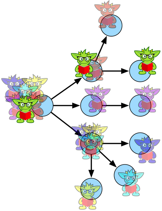
Interestingly, each traverser in Mr. v[69309689325]'s inbox had a name: Gyn$2345, Gyn$45, Gyn$93, etc. Gyn was a discrete particle of her wave function. Metaphysically speaking, Gyn was actually following the advice of Yogi Berra: "If you come to a fork in the road, take it." That is, never sample(1). Her "particle self" chose one and only one path. However, her "wave self" was taking all paths. In this way, Gyn's x-memory was recording the collective experience of all versions of her self across the graph.
|
gremlin> hdfs.copyFromLocal('/tmp/wikipedia.kryo','wikipedia.kryo')
==>null
gremlin> graph = GraphFactory.open('conf/hadoop/wikipedia.properties')
==>hadoopgraph[gryoinputformat->gryooutputformat]
gremlin> g = graph.traversal(computer(SparkGraphComputer))
==>graphtraversalsource[hadoopgraph[gryoinputformat->gryooutputformat], sparkgraphcomputer]
gremlin> x = g.V().has('name','Graph database').repeat(groupCount('x').by('name').out('href')).times(20).cap('x').next(); []
gremlin> x.size()
==>731
gremlin> x.sort{-it.value}[0..Graph theory=8605598306892530155
==>Relational database=8261042800088851351
==>Lookup table=6445010682474768007
==>Database=6197419607053064185
==>Graph database=5476792361544609153
==>Triplestore=5407594041286532360
==>Computer science=5393693263901041351
==>Graph=5211554445366262382
==>Directed graph=5137233761698039530
==>Mathematics=5132301689156216357
gremlin> hdfs.ls('output')
==>rwxr-xr-x daniel supergroup 0 (D) x
==>rwxr-xr-x daniel supergroup 0 (D) ~traversers
|
Section 3: The Non-Erratic Ergodic Eigenvector
Suppose the following traversal:
|
g.V().repeat(groupCount('x').out('href')).times(t).cap('x') // for t between [1,75]
|
Every time a traverser reaches a vertex, the vertex is incremented in the x hash map (groupCount('x')). Initially, the distribution of frequencies changes erratically. However, over time, it reaches a stationary distribution. It is "stable" because even though the counters keep increasing, the relative proportion of the counters stays the same. For instance, if vertex v[a] has a count of 12 and vertex v[b] has a count of 45, then when vertex v[a] has a count of 24, vertex v[b] will have a count of 90. Said in another way, the dynamic traversers generate a static probability distribution that defines the likelihood that a single traverser will be at any one vertex at some point in time t ≈ ∞ (i.e. an ergodic process).
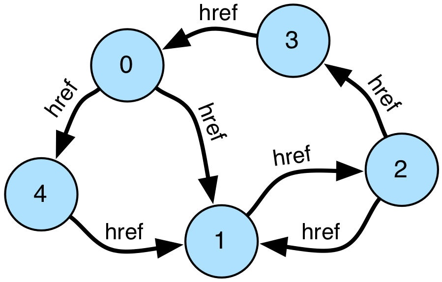 Assume the 5 vertex/7 edge graph diagrammed on the left. At g.V() (t=0), each vertex is provided one traverser. Each vertex increments its counter in x and then splits the traverser across its out('href')-adjacent neighbors. If the href-subgraph is strongly connected (i.e. reducible and non-transient) and lacks a compressable topology (i.e. aperiodic), then a stationary distribution is guaranteed to exist. That distribution, which can be normalized to a probability distribution (i.e. frequency / total frequency), is the graph's primary eigenvector. The primary eigenvector is typically used as a measure of each vertex's "centrality." For instance, given the diagrammed graph on the left, the primary eigenvector is [0.1308970114, 0.3442143899, 0.2493805577, 0.1806742088, 0.0948338322]. Thus, the ranking of the vertices from most central to least central is v[1], v[2], v[3], v[0], v[4] (one's eye seems to derive the same ranking).
| t | frequency | probability | distance from eigenvector |
|---|---|---|---|
| 1 | [1, 1, 1, 1, 1] | [0.2, 0.2, 0.2, 0.2, 0.2] | 0.1986073055597093 |
| 2 | [2, 4, 2, 2, 2] | [0.1666666667, 0.3333333333, 0.1666666667, 0.1666666667, 0.1666666667] | 0.11660026048581866 |
| 3 | [3, 7, 5, 3, 3] | [0.1428571429, 0.3333333333, 0.2380952381, 0.1428571429, 0.1428571429] | 0.06422748181719035 |
| 4 | [4, 12, 8, 6, 4] | [0.1176470588, 0.3529411765, 0.2352941176, 0.1764705882, 0.1176470588] | 0.03143659614218381 |
| 5 | [7, 17, 13, 9, 5] | [0.1372549020, 0.3333333333, 0.2549019608, 0.1764705882, 0.0980392157] | 0.01473943578762356 |
| ... | ... | ... | ... |
| 30 | [26400, 69424, 50296, 36440, 19128] | [0.1308952441, 0.3442148269, 0.2493752727, 0.1806751021, 0.0948395542] | 8.04890130266237E-6 |
| 31 | [36441, 95825, 69425, 50297, 26401] | [0.1308995686, 0.3442125946, 0.2493812615, 0.1806716501, 0.0948349252] | 4.242558551157544E-6 |
| 32 | [50298, 132268, 95826, 69426, 36442] | [0.1308957477, 0.3442148545, 0.2493780253, 0.1806745433, 0.0948368292] | 4.1616991553931435E-6 |
| 33 | [69427, 182567, 132269, 95827, 50299] | [0.1308982652, 0.3442133981, 0.2493811146, 0.1806730532, 0.0948341689] | 2.077160932619329E-6 |
| 34 | [95828, 251996, 182568, 132270, 69428] | [0.1308964745, 0.3442145091, 0.2493791747, 0.1806745072, 0.0948353345] | 2.13567485821227E-6 |
| 35 | [132271, 347825, 251997, 182569, 95829] | [0.1308977517, 0.3442138525, 0.2493807466, 0.1806735537, 0.0948340955] | 1.1709009180968303E-6 |
| ... | ... | ... | ... |
| 70 | [10478348120, 27554473290, 19962994332, 14463028872, 7591478958] | [0.1308970114, 0.3442143899, 0.2493805576, 0.1806742088, 0.0948338323] | 1.414213562373095E-10 |
| 71 | [14463028873, 38032821411, 27554473291, 19962994333, 10478348121] | [0.1308970114, 0.3442143899, 0.2493805577, 0.1806742087, 0.0948338322] | 1.0E-10 |
| 72 | [19962994334, 52495850286, 38032821412, 27554473292, 14463028874] | [0.1308970114, 0.3442143899, 0.2493805577, 0.1806742088, 0.0948338323] | 1.0E-10 |
| 73 | [27554473293, 72458844621, 52495850287, 38032821413, 19962994335] | [0.1308970114, 0.3442143899, 0.2493805577, 0.1806742088, 0.0948338322] | 0.0 |
| 74 | [38032821414, 100013317916, 72458844622, 52495850288, 27554473294] | [0.1308970114, 0.3442143899, 0.2493805577, 0.1806742088, 0.0948338322] | 0.0 |
| 75 | [52495850289, 138046139331, 100013317917, 72458844623, 38032821415] | [0.1308970114, 0.3442143899, 0.2493805577, 0.1806742088, 0.0948338322] | 0.0 |
Unbeknownst to Gyn, The Graph (eigen) was using her(selves) to sort itself (vector). Why was it doing this? The Graph represents its vertices and edges in a 512-bit address space (2512 = 1.34×10154). Unfortunately, the ever present Big and Small Traversals (as well as the countless other traversals executed since) have pushed The Graph close to the limits of representation. In order to avoid inconsistencies, The Graph needed to prune itself. To do this, it decided it best to destroy those vertices which were contributing little to its overall structure. Like cutting one's finger nails, The Graph began a systematic process of cosmic proportions to delete all peripheral vertices (and their respective incident edges). The Graph was forgetting in order to specialize its structure for a purpose that was beyond the realization of the vertices and traversers. Within The Graph's conceptual subgraph, knowledge worker traversers wandered through the morass of concept vertices and, in a collective self-similar manner, aided The Graph in its determination of which aspects of it's structure were worth preserving (and ultimately, extending). Gyn's passion for knowledge was simply an innate predisposition. Her happiness was not a function of her own being, but instead, of The Graph's will -- a carrot for her devotion. Gyn was part of a larger computation. In order to escape the dark sense that her life was not hers and hers alone, she began the long arduous journey towards realizing that she is, and always has been, The TinkerPop.
Credits
Written by Marko A. Rodriguez
Data and Result Generation by Daniel Kuppitz
Artwork by Ketrina Yim
Graph Visualizations by Daniel Kuppitz
Explanatory Diagrams by Marko A. Rodriguez
Gremlin Traversal Development by Daniel Kuppitz
Experimental Design by Marko A. Rodriguez
Executive Producer: Robin Schumacher
Undirected Edge #42 as himself
Russian Language Advisor: Pavel Yaskevich
Tamil Language Advisor: Harihar Shankar
Hindi Language Advisor: Swetha Sharma
Inspired by The Hitchhiker's Guide to the Galaxy and Flatland
Special thanks to DataStax and Apache TinkerPop.
No traversers were harmed during the making of this story.
Chapter 1: Life and Fate by Grasily Gremssman
Chapter 2: Permutation City by Grem Egrem
Section 1: The Birth of the Graph
Section 2: Graphialsynthesis and the Emergence of the Directed, Labeled Graph
Section 3: On the Baselessness of the Multi-MultiGraph
Chapter 3: A Mathematician's Apology by G.H. Gremdy
Section 1: Traversal Optimization via Algebra
Section 2: Traversal Optimization via Indices
Section 3: Traversal Optimization via Bulking
Chapter 4: Cognition in the Wild by Gredwin Grutchins
Chapter 5: We the Living by Gyn Grand
Section 1: Prelude to the Illusion of Freedom
Section 2: The Structure-Process Duality in Computing
Section 3: The Non-Erratic Ergodic Eigenvector
Credits
More Company
View All
London Called. RAG++, The AI Event, Answered!

DataStax Named a Leader in The Forrester Wave™: Vector Databases, Q3 2024

Live From New York! It’s RAG++, The AI Event