Vector Search for Production: A GPU-Powered KNN Ground Truth Dataset Generator

DataStax Astra DB and Apache Cassandra have always treated performance and scalability as first class citizens. When building Astra DB's vector search capabilities and its underlying ANN library (jvector), we spent a lot of time and energy optimizing for recall and precision in addition to the traditional database performance characteristics we’re used to dealing with (latency and throughput). 

Unfortunately, the datasets in common use for validating vector search recall predate the use of large ML models for vector similarity embeddings. Most are under 100 dimensions, while small general purpose embedding models start at 384 dimensions.

Thus, we found ourselves in the business of creating ground-truth KNN datasets that were more representative of these larger embeddings models. The tool we created to do this using GPU acceleration is called Neighborhood Watch (nw).

Here, we’ll share our motivation for releasing the tool, a configurable GPU-powered ground truth KNN dataset generator with a wide spectrum of embedding models. It addresses limitations in existing KNN datasets and we foresee its usefulness in computing KNN ground truth for custom datasets.

(If you're just here for the tooling/code, the GitHub repo is here.)

A quick overview of KNN, ANN, and recall 

For the purposes of this post, we won’t get into a deep discussion on the various recall and precision metrics relevant for vector stores, but it is worthwhile to do a quick recap of why we even care about things like recall and KNN ground truth to begin with. 

Deep neural networks and LLMs have made it possible to encode the semantic meaning of things (images, chunks of text, etc.) into lists of floats (vectors). These vectors are known as embeddings, and they are usually generated by running inference for some input on a neural net and using the output of one of the hidden layers as the embedding. The models are trained so that embeddings for things that are related (like the words cat and dog) will end up closer to each other in vector space, and things that are unrelated (like the words cat and bodybuilder) do not. 

We can determine how close two vectors are to each other by calculating their cosine distance, which, in its simplest form (for normalized vectors), is just the dot product of the vectors.

A ⋅ B = a1×b1 + a2 × b2​+⋯+an×bn

Let's do a quick example:

   A=[0.5959,0.3442,0.7256]

   B=[0.6769,0.3783,0.6314]

A ⋅ B =(0.5959×0.6769)+(0.3442×0.3783)+(0.7256×0.6314) = 0.9917

In this example, A is quite close to B because their similarity (dot product) is almost 1. (A dot product of 1.0 would mean they are the same [normalized] vector.) For any pair of vectors with dimensions D, we can obtain their similarity with D multiplications and additions, i.e. the complexity of this calculation is O(D).

The goal of a vector store is to take a query vector and quickly fetch the most similar vectors from a large, changing dataset of vectors. We could naively go about doing this by calculating the distance between the query vector and each vector in the dataset that can be described as having linear complexity in the number of stored vectors‚specifically O(N), where N is the number of the size of the dataset. 

More precisely, for 10,000 query vectors, a dataset of 1 million vectors, and 1,536 dimensions we would have to do 10k * 1M = 10B similarity comparisons, and because each similarity comparison involves 1,536 computations, we'd have to perform 1.536 trillion calculations.

If you have an image of some two-dimensional points in your mind's eye, you may wonder if we can't just look at the right part of the vector space and reduce the amount of distance calculations we have to do. We can! There are data structures like k-d trees that help with precisely this problem. Building k-d trees has O(D x N log N) complexity and searching them also has O(D x N log N). Unfortunately, this only holds for lower values of D. For larger values of D, the query time complexity degrades to O(D x N) and so the total cost can be worse than the brute force approach, which requires no "training or indexing".

So what do we do? Since most vector search use cases do not require exact results, we attempt to scale KNN by giving up some precision.This is called ANN, for approximate nearest neighbors. If we query Honeycrisp apples and we get Macintosh instead of Red Delicious it might not matter–in fact, a bit of inexactness is sometimes a feature in generative AI use cases (see things like temperature in NLP). Additionally, in RAG (retrieval augmented generation) use cases, large language models seem to be able to select only the most relevant data when encouraged via a prompt.

Clearly, however, there is a limit to this sort of logic (we wouldn't want the apple query to return a dog breed) and we need objective measures to determine the quality of our ANN. Our measure(s) should account for how many of the true top K neighbors our search returns. We may also care about ensuring that these results come in the right order. Regardless of the exact measure(s) we use, it's clear that in order to test the quality of our ANN we need to test it against large, representative, ground truth KNN datasets.

Note: when we say true top K neighbor, we’re talking about the mathematically closest vertex in the dataset, not a subjective interpretation of the most similar thing in the dataset. If we start talking about human interpreted similarity, we are no longer measuring the quality of the ANN, we are measuring the quality of the embedding.

But why build our own datasets?

The complexity of generating KNN for large datasets is high (O(Q×D×N), as described above, so the naive approach would be to leverage publicly available, generally accepted datasets. The two most famous sets of KNN datasets can be found at  erikbern/ann-benchmarks:

and and at big-ann-benchmarks:

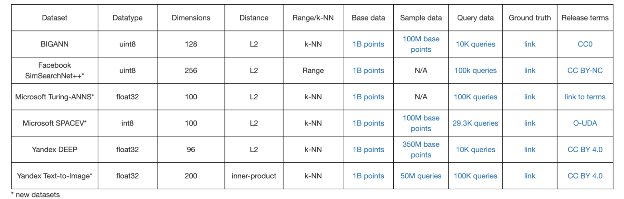
We found that the ann-benchmark datasets are great for local testing or short runs, but both these and the big-ann datasets have relatively low dimensionality. This makes them of limited use for benchmarking real-world vector embeddings workloads. As of late 2023, the most popular text embeddings model we see is ada-002, a 1,536-dimension embeddings model. Even a small model like the open-source e5 model is 384 dimensions. Similarly, image / multi-modal workloads involve CLIP embeddings which depending on the size / patch can be 512, 768, or 1,024.

We created Neighborhood Watch to create ground truth datasets for high-dimension embeddings vectors that are more representative of what people are actually using today.

The Neighborhood Watch project

Overview

Generating a ground truth datasets involves five phases: 

1. Data preparation - extracting and splitting chunks from large, representative datasets for the base and query vectors
2. Embedding generation - supporting both local and api based models
3. Computing KNN - using a brute-force approach
4. Exporting the final dataset - including the resulting distances, indices, and vectors in a consumable format
5. Validation - ensuring that the generated nearest neighbors are valid by comparing distances using a manual cpu based computations

The neighborhood watch project incorporates GPU acceleration to execute the aforementioned five steps and generate ground truth KNN datasets. 

It began as a series of Python scripts, but we cleaned it up and added a CLI for ease of use. The Python library dependency of this project is managed by poetry (which you need to install first before you can run the CLI program).

The command line interface was designed to be configurable and allows the options in the code block below. It is worth pointing out that the dimensionality is automatically inferred from the model being used. For example, text-embedding-ada-002 model output has 1,536 dimensions and textembedding-gecko model’s output dimension is 768.

In the following sections, we'll go over design decisions and unexpected findings for each of the five phases. The entire pipeline supports out-of-core datasets via chunking, and leverages GPUs where appropriate.

Note: it is surprisingly non-trivial to set up the Python environment to run this program. We’ll cover the environment setup with more details in Appendix A.

Data preparation

In order to run realistic benchmarks, we wanted to ensure we had a large enough dataset that was diverse and representative of the sort of datasets we see in RAG. We also wanted to ensure that we had realistic query vectors that were neither randomly generated nor simply a subset of the data vectors. Finally, we wanted to ensure that we supported multiple embedding models (both open source and proprietary). 

There are many large, useful text datasets available in Hugging Face datasets  so we built Neighborhood Watch to automatically download Hugging Face datasets using their datasets library. 

In our first implementation we generated query vectors from the same dataset as the base vectors and simply split them a different way so as to get different but related vectors, but we eventually decided to use purpose-built datasets to achieve more realistic queries. We settled on the Wikipedia and squad datasets to generate base and query vectors, respectively. A future version might allow users to bring their own datasets, either by picking existing Hugging Face datasets or providing their own in a format like Parquet or Arrow IPC.

The strategy used to split or chunk text documents can make a significant difference in RAG quality. We landed on using spaCy sentence splitter for a few reasons:

1. Sentences are relatively smaller chunks and this allows us to play nice with the token limits of a variety of models
2. Smaller chunks result in more embeddings, which allows us to do bigger KNN datasets with the same Wikipedia data
3. SpaCy has relatively simple dependencies compared to LangChain and LlamaIndex, and we preferred to use a standard solution instead of inventing a new one
4. We believe that relatively small embeddings for the search part of RAG, with a slightly larger return dataset, are more effective. This could be done efficiently by returning the sentences around the result rather than by using techniques like chunk overlap

Generating embeddings

Generating embeddings is very expensive, and for smaller data sets it's by far the slowest part of the process (this changes as the datasets get large). 

We found that batching is the most important lever in embedding performance both for online and offline models and tried to find sweet spots for each model. This makes sense because batching allows us to better use GPUs during inference. We found that we needed different batch settings for each embedding model. 

• VertexAI Gecko was the easiest because they have a maximum batch value of 250. Otherwise, the VertexAI API will return an error. 
• OpenAI is the tricky one because they limit their requests by tokens, so the number of batches you can pass depends on the data itself. In our testing with the Wikipedia source dataset, we landed with the batch size of 50 sentences without hitting the input token limit (with only very few noticed exceptions).
• For open-source models we settled on a batch size of 1,000 sentences. 

In our testing, we also noticed that OpenAI could throw some content / safety moderation errors when making embeddings, resulting in failure. We reproduced the issue in this gist.

For cases where the model failed to generate the embeddings, we originally inserted zero vectors into the dataset. But this may cause problems when we do an ANN query, since the cosine with a zero vector is undefined. We therefore added the CLI parameter [--skip-zero-vec | --no-skip-zero-vec] (default is skip zero vector) to give you an option here.

After completing this phase, the raw, source datasets (squad and Wikipedia), along with the generated embeddings, are saved in two separate files using the Parquet file format.

Computing KNN

Given that computing the distance between vectors is an embarrassingly parallelizable problem, we looked to GPUs to do the heavy lifting. We eventually landed on the Nvidia RAFT (Reusable Accelerated Functions and Tools) library to perform the actual KNN.  

Over the past few years Nvidia has invested in developing GPU-accelerated algorithms and primitives for AI in their RAFT library. Recently (this year), they have rebranded it as primarily a vector search library (Reusable Accelerated Functions and Tools for Vector Search and More). This library is consumed downstream by other libraries in the RAPIDS ecosystem such as the cuML library, etc.

We actually started by using cuML's cuml.neighbors.NearestNeighbors with the brute algorithm but we ran into a couple of correctness bugs (cuml-pr-3304 and cuml-issues-5569) which led us to using the RAFT pylibraft.neighbors API directly. In particular, the brute force KNN method is used:

from pylibraft.neighbors.brute_force import knn

distances, neighbors = knn(dataset, queries, k)

The central aspect of this program lies in this phase, and thanks to the RAFT library, the implementation of KNN calculation becomes notably straightforward. Challenges primarily arise from a few other areas.

Effective GPU memory use

In this step, the query and base vector dataset (and their embeddings) are processed in batches. The batch size, however, can be dynamically tuned based on the available GPU memory and the actual memory utilization. This is controlled by the --enable-memory-tuning or --disable-memory-tuning CLI input parameter. 

When memory tuning is turned off, the batch size remains constant at 100,000. Conversely, when enabled, the program dynamically adjusts the batch size—increasing or decreasing—if the memory utilization exceeds a predefined threshold (10% of the total GPU memory).

This program facilitates an additional optimization through the --use-dataset-api | --no-use-dataset-api option. The distinction lies in choosing between the Apache Arrow (pyarrow) Table API or Dataset API. The program defaults to using the Table API, but the Dataset API should be selected for larger-than-memory computations

Exporting the final dataset 

The KNN stage outputs the KNN indices and distance vectors, determined through brute force KNN calculations, employing the query dataset, base dataset, and the specified number of neighbors to return (K). These datasets, along with subsets of the query vectors and base vectors sourced from the raw Squad/Wikipedia datasets (along with their embeddings), are individually stored in four distinct files using the Parquet file format. 

The program also has the following two CLI options to control the final dataset exporting behavior:

• The -d (--data_dir) <data_dir_name> option controls where to put the generated final datasets. If not specified, it defaults to the knn_dataset subfolder.
• The --gen-hdf5 | --no-gen-hdf5 option facilitates the creation of a consolidated dataset in HDF5 format, grouping the contents of the aforementioned four files together. In the absence of specific instructions, the default behavior is to generate the supplementary HDF5 format file.

Post validation

Finally, the program provides the option to verify the accuracy of the generated KNN dataset using either the --post-validation | --no-post-validation flags. 

In the post-validation process, each query vector is iterated over, its similarity (dot product) with the corresponding base vector is calculated, and the result is compared with the corresponding KNN distance vector. The mismatch count is incremented in case of a discrepancy. Upon completion of this process, the total mismatch count is displayed. 

Due to its time-consuming nature, the post-validation process is disabled by default. But when working with custom datasets it's advisable to first enable this option on a smaller dataset before trying out the nw program on a larger one, thus preventing wasted time and resources on unusable results.

Summary

In this blog post, we have introduced a GPU-powered generator, neighborhood watch (nw), designed for conducting exhaustive KNN dataset computations across a spectrum of embedding models. This unveiling is a significant stride in our ongoing efforts to enhance the vector search capabilities of Astra DB. With confidence in nw's configurability and compatibility with diverse datasets and models, users can expect precise KNN computations tailored to their unique datasets. Please check out the GitHub repo here.

Appendix: Set up the execution environment

To get started, make sure you have a Linux host with GPU cards. You'll need Python version 3.10 (other versions won't work), and it's recommended to use Conda or VirtualEnv for optimal setup.

Once your virtual environment with Python 3.10 is set up, install dependencies with the command: poetry install.

Our pyproject.toml file is configured for CUDA Toolkit 12.2 (compatible with version 12.3, but some adjustments may be needed due to possible dependency version changes).

For a quick setup, check out our GitHub repository with helpful scripts:

• For bare-metal systems, use the bash script install_baremetal_env.sh (tested on an EC2 instance with Ubuntu 22.04).

If you prefer containerized installation, use the provided Dockerfile to create an image with all necessary requisites for an efficient setup.