Understanding Hierarchical Navigable Small Worlds (HNSW)

What are Hierarchical Navigable Small Worlds (HNSW)?

Introduced in a 2016 paper, Hierarchical Navigable Small World (HNSW) is more than just an acronym in the world of vector searching; it's the algorithm that underpins many vector databases. Available under the Apache Lucene project and other implementations, what makes HNSW stand out from other vector indexing techniques is its approach to tackling a common challenge in data science and artificial intelligence: efficiently finding the nearest neighbors in large multi-dimensional datasets.

In a nutshell, HNSW creates a multi-layered graph structure where each layer is a simplified, navigable small world network. A mental analog you may consider is that of a digital map of a road network. Zoomed out, you see how cities and towns are connected by major roads. Zoom in to the city level, and you can see how people within that city connect to each other. At the finest level of zoom, you can see how neighborhoods and communities are interconnected.

Similarly, HNSW constructs layers of connections with varying degrees of reachability. This structure allows for remarkably quick and accurate searches, even in vast, high-dimensional data spaces. This post will explore some of the inner workings of HNSW, along with some of its strengths and weaknesses.

Why are Hierarchical Navigable Small Worlds Important?

Hierarchical Navigable Small Worlds are important as they provide an efficient way to navigate and search through complex, high-dimensional data. This structure allows for faster and more accurate nearest-neighbor searches, essential in various applications like recommendation systems, image recognition, and natural language processing. By organizing data hierarchically and enabling navigable shortcuts, HNSW significantly reduces the time and computational resources needed for these searches, making it a crucial tool in handling large datasets in machine learning and AI.

Understanding Similarity Search

Similarity search is a fundamental technique in data science, used to find data points in a dataset that are 'nearest' to a given query; as these searches are often within a vector space, it is also known as “vector search”. Such searches are used by systems such as voice recognition, image / video retrieval, and recommendation systems (amongst others); more recently it has been brought to the forefront of generative AI as one of the main drivers to improve performance through Retrieval-Augmented Generation (RAG).

Traditionally, methods like brute-force search, tree-based structures (e.g., KD-trees), and hashing (e.g., Locality-Sensitive Hashing) were used. However, these approaches do not scale well with large, high-dimensional datasets, leading to the need for more efficient solutions. A graph-based approach called Navigable Small World (NSW) improved on the scaling abilities of its predecessors, but this ultimately has polylogarithmic scaling characteristics, limiting its utility in large-scale applications where there are a large number of both records and dimensions.

This is where Hierarchical Navigable Small World (HNSW) enters the frame - it builds on NSW by introducing layers (“hierarchies”) to connect data, much like adding a “zoom out” feature to a digital map.

Underpinnings of HNSW

Before going further on HNSW, we should first explore the Navigable Small World (NSW) and a data structure called “skip lists”, both of which make use of a graph-based data structure. In such a structure, the data (nodes) are connected to each other by edges, and one can navigate through the graph by following these edges.

Navigable Small Words (NSW)

The principle behind Navigable Small Worlds is that every node can be reached within a small number of “hops” from any other node. After determining an entry point (which could be random, heuristic, or some other algorithm), the adjacent nodes are searched to see if any of them are closer than the current node. The search moves to the closest of these neighboring nodes and repeats until there are no closer nodes.

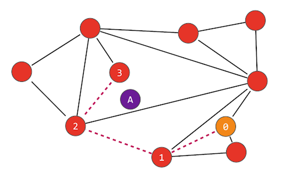
In the following illustration, we are searching for the node nearest to “A”, and start by looking at node “0”. That node is connected to three nodes, but the one that is closest to “A” is node “1”. We then repeat the process from node “1”, finding that node “2” is closer than node “1”, and finally that node “3” is closer than node “2”. The nodes connected to “3” are all further away from “A”, so we determine that “3” is the closest node:

In building the graph, the M parameter sets out the number of edges a new node will make to its nearest neighbors (the above example uses M=2). A larger M means a more interconnected, denser graph but one that will consume more memory and be slower to insert. As nodes are inserted into the graph, it searches for the M closest nodes and builds bidirectional connections to those nodes. The network nodes will have varying degrees of connectivity, in a similar fashion to how social networks contain users connected to thousands (or millions) of people and others that are connected to hundreds (or tens) of people. An additional Mmax parameter determines the maximum number of edges a node can have, as an excessive number of edges can affect performance.

One of the shortcomings of NSW search is that it always takes the shortest apparent path to the “closest node” without considering the broader structure of the graph; This is known as “greedy search”, and can sometimes lead to being trapped in a local optimum or locality – a phenomenon known as “early stopping”. Consider what might happen in the following diagram, where we enter at a different node “0” with a different “A” node:

The two nodes connected to node “0” are both further away from “A”, so the algorithm determines that “0” is the closest node. This can happen at any point during the navigation, not just the starting node. It does not try to explore branches beyond any nodes that are further away, as it assumes anything further away is even further away! There are techniques to mitigate this, such as testing multiple entry points, but they add to cost and complexity.

Skip Lists

The structure of a skip list allows both insertion and querying operations to be performed on the order of average O(log n) – the time of the operation grows logarithmically with the amount of data, rather than linearly, polylogarithmically, or worse. At the bottom of a skip list, every node is connected to the next node in order. As more layers are added, nodes in the sequence are “skipped”. The following Wikipedia illustration shows how ten nodes might be organized into a four-layer skip list:

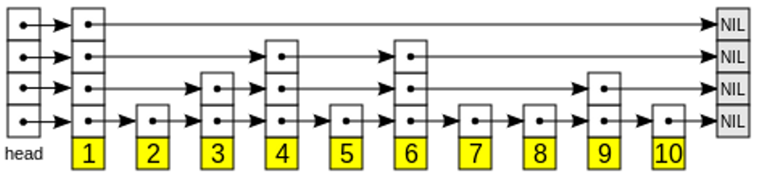
Skip lists are generally built probabilistically - the likelihood of a node appearing in a layer decreases at higher layers, which means the higher layers have fewer nodes. When searching for a node, the algorithm enters at the “head” of the top layer and proceeds to the next element that is greater than or equal to the target. At this point, the search element is found, or it drops to the next (more fine-grained) layer, and the process repeats until you’ve either found the search node, or you’ve found the adjacent nodes to your search node. Within the context of skip lists and similarity search, “greater than” means “more similar” - in the case of cosine similarity, for example, the closest you can get would be a similarity of 1.

Insertion involves determining what layer the node is to enter the structure, seeking to the first node that is “greater than” but keeping track of the last node before the “greater than” node. Once it finds that “greater than” node, it updates the last node to point at the new node, and points the new node to the “greater than” node. It then proceeds to the next layer down, until the node appears in all layers. Deletions follow a similar logic to locating and updating pointers.

Introducing Hierarchical Navigable Small Worlds (HNSW)

Transitioning from Navigable Small World (NSW) to Hierarchical Navigable Small World (HNSW) marks a shift from polylogarithmic complexity to streamlined logarithmic scaling in vector searches. HNSW marries the swift traversal of skip lists with NSW’s rich interconnectivity, adding a hierarchical twist for enhanced search efficiency.

At the heart of HNSW is its tiered architecture, which organizes data into layers of interconnected nodes, allowing rapid skips across unnecessary computations to focus on pertinent search areas. This hierarchical approach, coupled with the small-world concept, optimizes the path to high-precision results, essential for applications demanding quick and accurate retrievals.

HNSW not only simplifies the complexity of navigating large datasets but also ensures consistent and reliable performance, underscoring its prowess in modern data-intensive challenges.

How HNSW works

Let’s go down a layer and discuss how HNSW works in more detail, including both the building and maintenance of the index, as well as conducting searches within the index.

Building the hierarchical structure

The foundation of HNSW lies in its hierarchical structure. Building this multi-layered graph starts with a base layer that represents the entire dataset. As we ascend the hierarchy, each subsequent layer acts as a simplified overview of the one below it, containing fewer nodes and serving as express lanes that allow for longer jumps across the graph.

The probabilistic tiering in HNSW, where nodes are distributed across different layers in a manner similar to skip lists, is governed by a parameter typically denoted as mL. This parameter determines the likelihood of a node appearing in successive layers, with the probability decreasing exponentially as the layers ascend. It's this exponential decay in probability that creates a progressively sparser and more navigable structure at higher levels, ensuring the graph remains efficient for search operations.

Constructing the navigable graph

Constructing the navigable graph in each layer of HNSW is key to shaping the algorithm's effectiveness. Here, the parameters M and Mmax, inherited from the NSW framework, play a crucial role. A new parameter Mmax0 is reserved for the ground layer, allowing for greater connectivity at this foundational level than at the higher levels. HNSW also adds the efConstruction parameter, which determines the size of the dynamic candidate list as new nodes are added. A higher efConstruction value means a more thorough, albeit slower, process of establishing connections. This parameter helps balance connection density, impacting both the search's efficiency and accuracy.

An integral part of this phase is the advanced neighbor selection heuristic, a key innovation of HNSW. This heuristic goes beyond simply linking a new node to its nearest neighbors; it also identifies nodes that improve the graph's overall connectivity. This approach is particularly effective in bridging different data clusters, creating essential shortcuts in the graph. This heuristic, as illustrated in the HNSW paper, facilitates connections that a purely proximity-based method might overlook, significantly enhancing the graph's navigability:

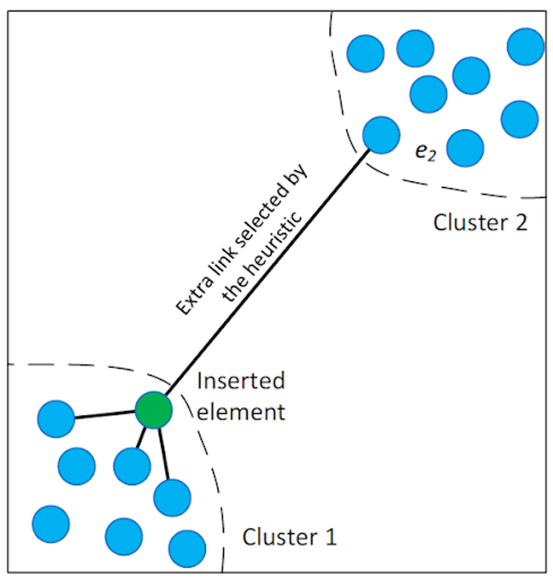
By strategically balancing connection density and employing intelligent neighbor selection, HNSW constructs a multi-layered graph that is not only efficient for immediate searches but is also optimally structured for future search demands. This attention to detail in the construction phase is what enables HNSW to excel in managing complex, high-dimensional data spaces, making it an invaluable tool for similarity search tasks.

Search process

Searching in HNSW involves navigating through the hierarchical layers, starting from the topmost layer and descending to the bottom layer, where the target's nearest neighbors are located. The algorithm takes advantage of the structure's gradation – using the higher layers for rapid coarse-grained exploration and finer layers for detailed search – optimizing the path towards the most similar nodes. Heuristics, such as selecting the best entry points and minimizing hops, are employed to speed up the search without compromising the accuracy of the results.

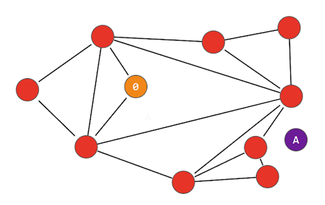
If we revisit our simple NSW example from above, we can see how the HNSW search process works. Looking for the nearest neighbor of node “A”, we start by picking a node on the top-most Layer 2 and navigating (as with NSW) to its nearest neighbor node “1”. At this point, we go down a layer to Layer 1, and search to see if this layer has any closer neighbors, which we find as node “2”. We finally go down to the bottom Layer 0, and find that node “3” is closest:

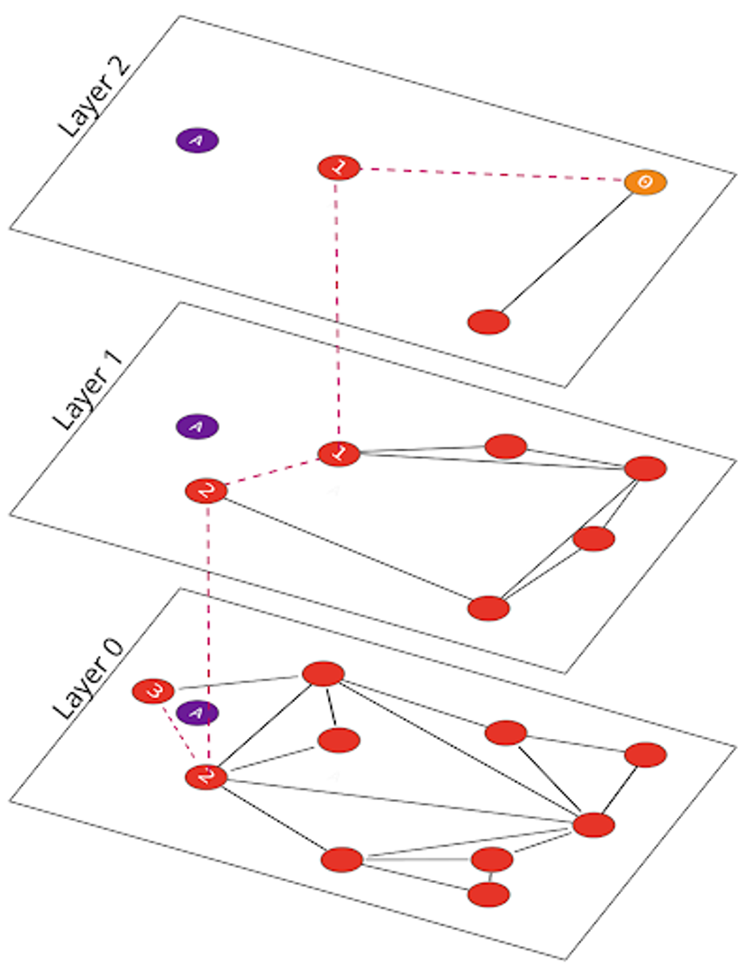
Searching within HNSW is similar to searching within NSW, with an added “layer” dimension that allows quick pruning of the graph to only those relevant neighbors.

Insertions and Deletions

Insertions and deletions in the Hierarchical Navigable Small World (HNSW) graph ensure its dynamic adaptability and robustness in handling high-dimensional datasets.

Insertions:

When a new node is added to the HNSW graph, the algorithm first determines its position in the hierarchical structure. This process involves identifying the entry layer for the node based on the probabilistic tiering governed by the parameter mL. The insertion starts from that layer, connecting the new node to the M closest neighbors within that layer. If a neighboring node ends up with more than Mmax connections, the excess connections are removed. The node is then inserted into the next layer down in a similar fashion, and the process continues to the bottom node where Mmax0 is referenced as the maximum connectivity.

Deletions:

The process of removing a node from an HNSW graph involves careful updating of connections, particularly in its neighbors, across multiple layers of the hierarchy. This is crucial to maintain the structural integrity and navigability of the graph. Different implementations of HNSW may adopt various strategies to ensure that connectivity within each layer is preserved and that no nodes are left orphaned or disconnected from the graph. This approach ensures the continued efficiency and reliability of the graph for nearest-neighbor searches.

Both insertions and deletions in HNSW are designed to be efficient while preserving the graph's hierarchical and navigable nature, crucial for the algorithm's fast and accurate nearest-neighbor search capabilities. These processes underscore the adaptability of HNSW, making it a robust choice for dynamic, high-dimensional similarity search applications.

Benefits and Limitations of HNSW

As with most any technology, for all the improvements HNSW brings to the world of vector search, it has some weaknesses that may not make it appropriate for all use cases.

Benefits of HNSW

• Efficient Search Performance: HNSW significantly outperforms traditional methods like KD-trees and brute-force search in high-dimensional spaces, as well as NSW, making it ideal for large-scale datasets.
• Scalability: The algorithm scales well with the size of the dataset, maintaining its efficiency as the dataset grows.
• Hierarchical Structure: The multi-layered graph structure allows for quick navigation across the dataset, enabling faster searches by skipping irrelevant portions of the data.
• Robustness: HNSW is known for its robustness in various types of datasets, including those with high dimensionality, which often pose challenges for other algorithms​​.

Limitations of H

• Memory Usage: The graph structure of HNSW, while efficient for search operations, can be memory-intensive, especially with a large number of connections per node. This imposes a practical limitation on graph size, as operations must be performed in memory if they are to be fast.
• Complex Implementation: The algorithm's hierarchical and probabilistic nature makes it more complex to implement and optimize compared to simpler structures.
• Parameter Sensitivity: HNSW performance can be sensitive to its parameters (like the number of connections per node), requiring careful tuning for optimal results.
• Potential Overhead in Dynamic Environments: While HNSW is efficient in static datasets, the overhead of maintaining the graph structure in dynamic environments (where data points are frequently added or deleted) could be significant.

In conclusion, while HNSW offers significant advantages in search efficiency and scalability, especially in high-dimensional spaces, it comes with trade-offs in terms of memory usage and implementation complexity. These factors must be considered when choosing HNSW for specific applications.

Try a Vector Database that has all of the benefits of HNSW

In this post, we have explored how HNSW has improved on its predecessors, enabling faster search for large multidimensional datasets. We’ve discussed how the HNSW graphs are built, searched, and maintained, and we have discussed some of the strengths and limitations of HNSW.

If you are looking for a vector database that keeps the strengths of HNSW, but eliminates the memory and concurrency problems found in many HNSW implementations, have a look at DataStax Vector Search, which uses the open source JVector project.

You can get started with DataStax Astra by registering here, and learn more about the non-vector capabilities of the NoSQL Astra platform here.