Sensor Data Modeling
Interested in learning more about Cassandra data modeling by example? This example demonstrates how to create a data model for temperature monitoring sensor networks. It covers a conceptual data model, application workflow, logical data model, physical data model, and final CQL schema and query design.

Conceptual Data Model
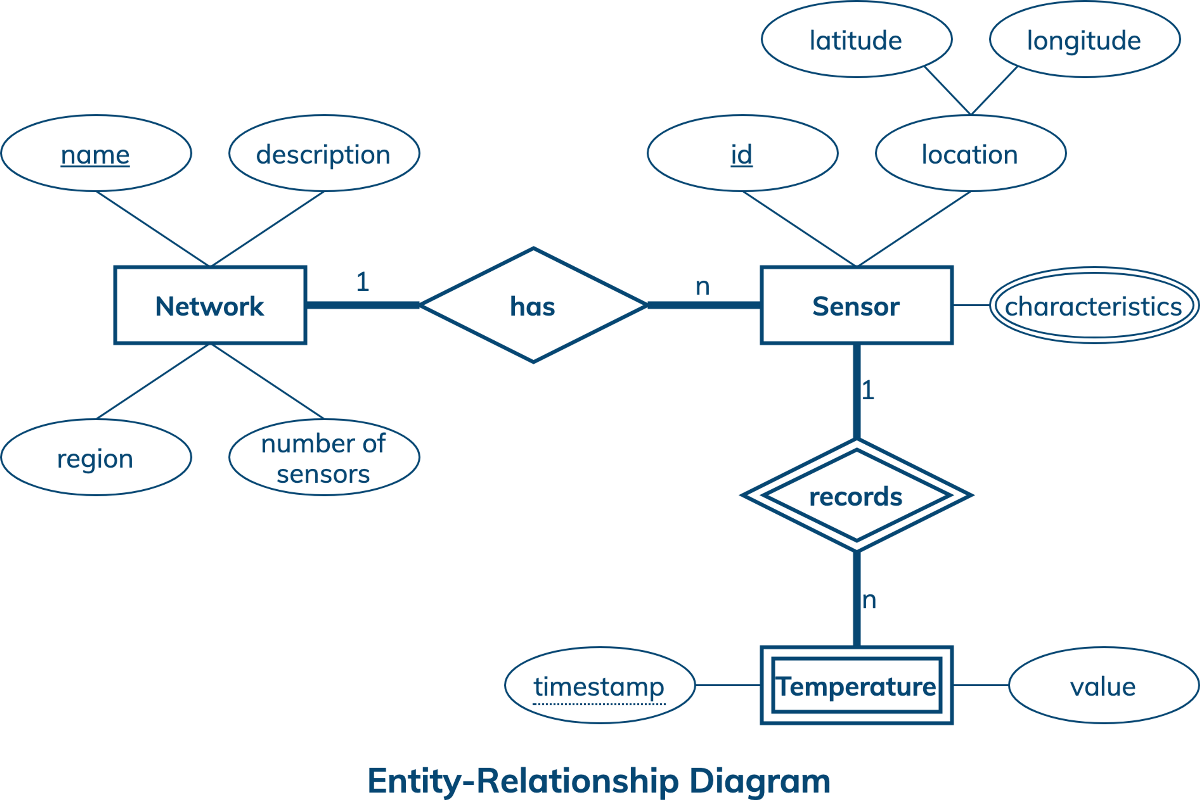
A conceptual data model is designed with the goal of understanding data in a particular domain. In this example, the model is captured using an Entity-Relationship Diagram (ERD) that documents entity types, relationship types, attribute types, and cardinality and key constraints.
The conceptual data model for sensor data features sensor networks, sensors, and temperature measurements. Each network has a unique name, description, region, and number of sensors. A sensor is described by a unique id, location, which is composed of a latitude and longitude, and multiple sensor characteristics. A temperature measurement has a timestamp and value, and is uniquely identified by a sensor id and a measurement timestamp. While a network can have many sensors, each sensor can only belong to one network. Similarly, a sensor can record many temperature measurements at different timestamps and every temperature measurement is reported by exactly one sensor.
Application Workflow
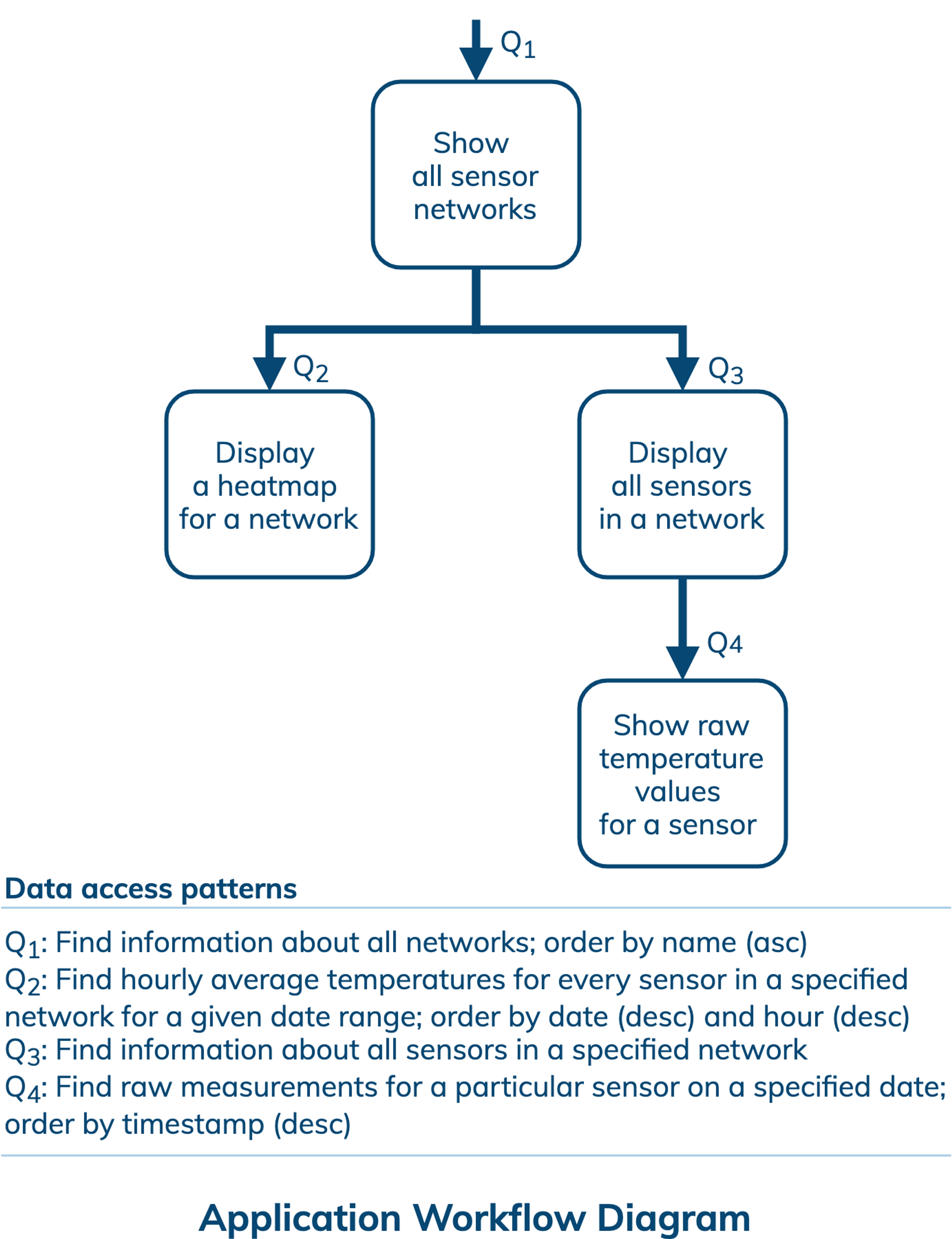
An application workflow is designed with the goal of understanding data access patterns for a data-driven application. Its visual representation consists of application tasks, dependencies among tasks, and data access patterns. Ideally, each data access pattern should specify what attributes to search for, search on, order by, or do aggregation on.
The application workflow has an entry-point task that shows all sensor networks. This task requires querying a database to find information about all networks and arrange the results in ascending order of network names, which is documented as Q1 on the diagram. Next, an application can either display a heatmap for a selected network, which requires data access pattern Q2, or display all sensors in a selected network, which requires data access pattern Q3. Finally, the latter can lead to the task of showing raw temperature values for a given sensor based on data access pattern Q4. All in all, there are four data access patterns for a database to support.
Next: Logical Data Model

Logical Data Model
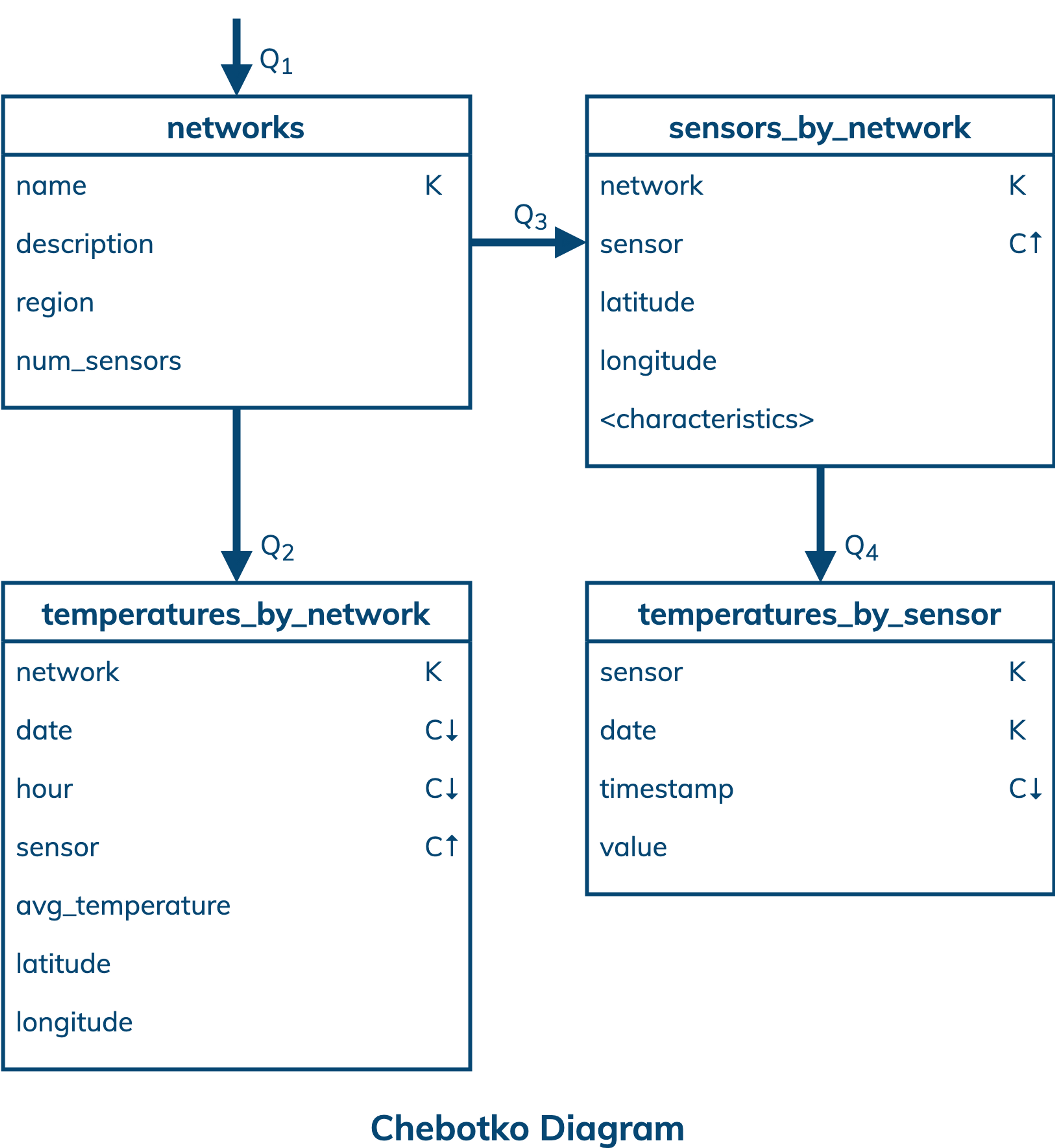
A logical data model results from a conceptual data model by organizing data into Cassandra-specific data structures based on data access patterns identified by an application workflow. Logical data models can be conveniently captured and visualized using Chebotko Diagrams that can feature tables, materialized views, indexes and so forth.
The logical data model for sensor data is represented by the shown Chebotko Diagram. There are four tables, namely networks, temperatures_by_network, sensors_by_network and temperatures_by_sensor, that are designed to specifically support data access patterns Q1, Q2, Q3 and Q4, respectively. For example, table temperatures_by_network has seven columns, of which network is designated as a partition key column, and date, hour and sensor are clustering key columns with descending or ascending order being represented by a downward or upward arrow. To support Q2, it should be straightforward to see that a query over this table needs to restrict column network to some value and column date to a range of values, while the result ordering based on date and hour is automatically supported by how data is organized in the table.
Next: Physical Data ModelPhysical Data Model
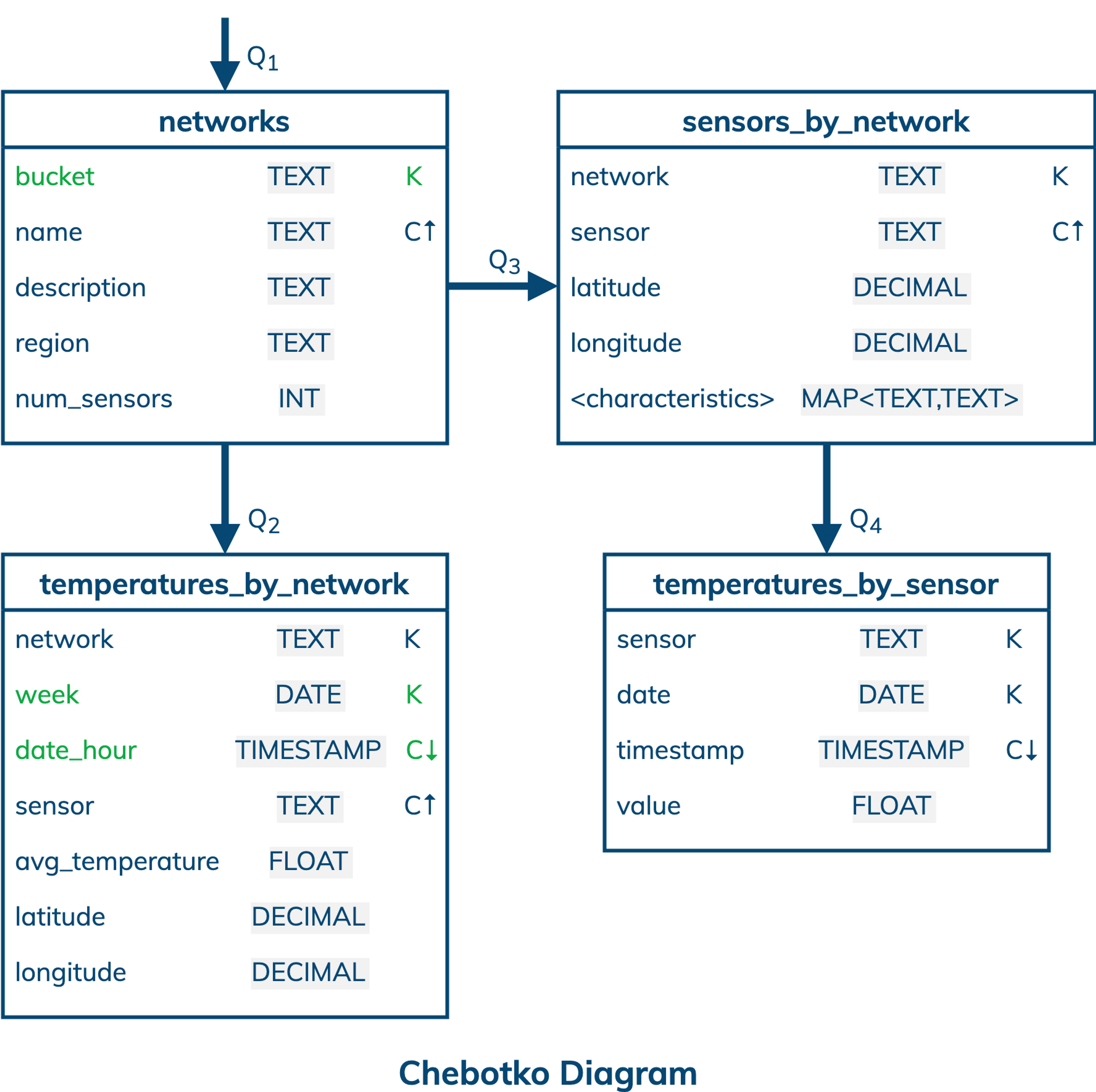
A physical data model is directly derived from a logical data model by analyzing and optimizing for performance. The most common type of analysis is identifying potentially large partitions. Some common optimization techniques include splitting and merging partitions, data indexing, data aggregation and concurrent data access optimizations.
The physical data model for sensor data is visualized using the Chebotko Diagram. This time, all table columns have associated data types. In addition, two tables have changes in their primary keys. Table networks used to be partitioned based on column name and is now partitioned based on column bucket. The old design had single-row partitions and required retrieving rows from multiple partitions to satisfy Q1. The new design essentially merges old single-row partitions into one multi-row partition and results in much more efficient Q1. With respect to table temperatures_by_network, there are two optimizations. The minor optimization is to merge columns date and hour into one column date_hour, which is supported by the TIMESTAMP data type. The major optimization is to split potentially large partitions by introducing column week, which represents the first day of a week, as a partition key column. Consider that a network with 100 sensors generates 100 rows per hour in table temperatures_by_network. The old design allows partitions to grow over time: 100 rows in an hour, 2400 rows in a day, 16800 rows in a week, …, 876000 rows in a year, and so forth. The new design restricts each partition to only contain at most 16800 rows that can be generated in one week. Our final blueprint is ready to be instantiated in Cassandra.
Skill Building
Skill Building
Want to get some hands-on experience? Give our interactive lab a try! You can do it all from your browser, it only takes a few minutes and you don’t have to install anything.
More Resources
Review the Cassandra data modeling process with these videos