Shopping Cart Data Modeling
Interested in learning more about Cassandra data modeling by example? This example demonstrates how to create a data model for online shopping carts. It covers a conceptual data model, application workflow, logical data model, physical data model, and final CQL schema and query design.

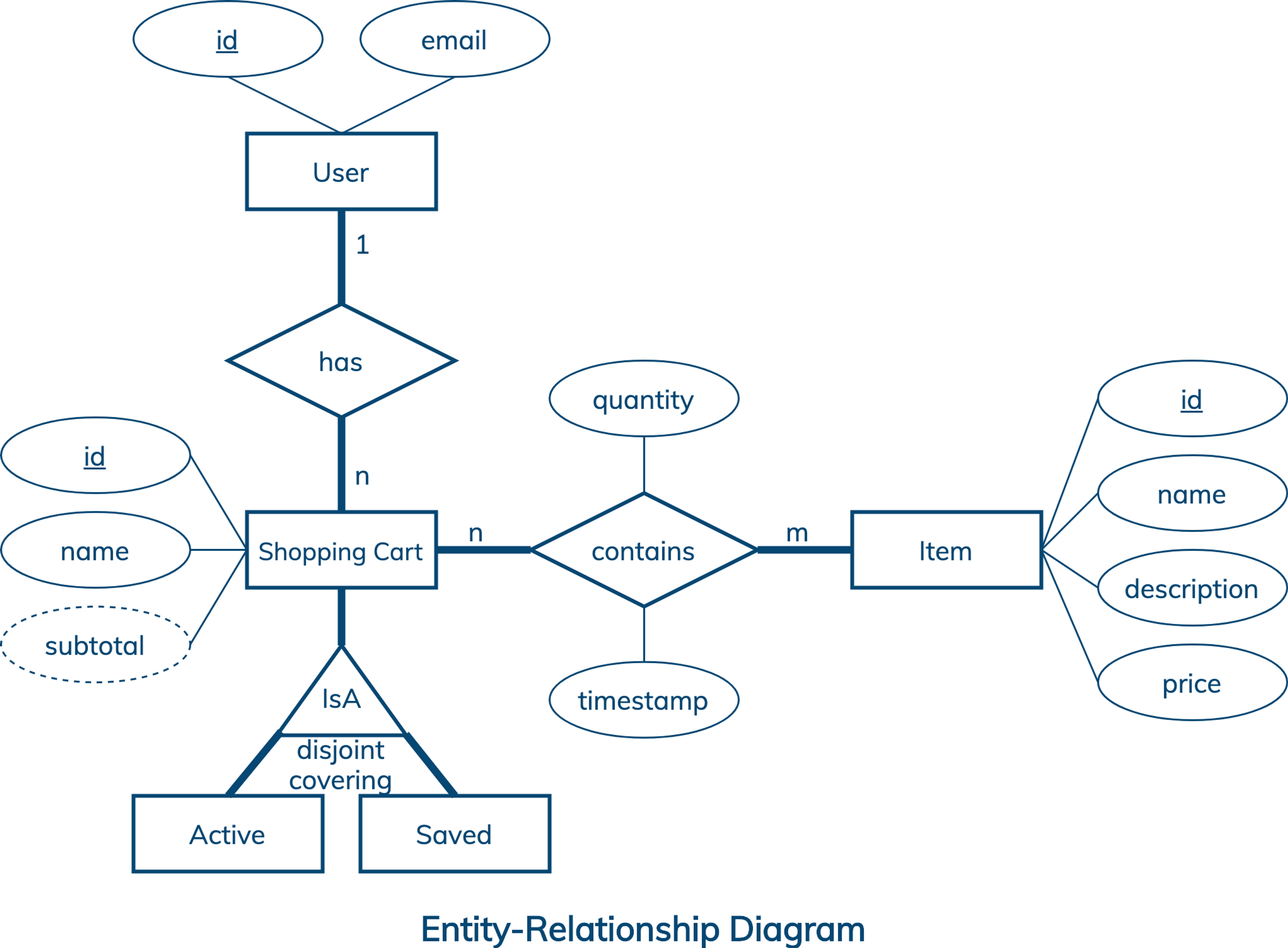
Conceptual Data Model
A conceptual data model is designed with the goal of understanding data in a particular domain. In this example, the model is captured using an Entity-Relationship Diagram (ERD) that documents entity types, relationship types, attribute types, and cardinality and key constraints.
The conceptual data model for shopping cart data features users, items and shopping carts. A user has a unique id and may have other attributes like email. An item has a unique id, name, description and price. A shopping cart is uniquely identified by an id and can be either an active shopping cart or a saved shopping cart. Other shopping cart attribute types include a name and subtotal. The latter is a derived attribute type whose value is computed based on prices and quantities of all items in a cart. In general, a derived attribute value can be stored in a database or dynamically computed by an application. While a user can create many shopping carts, each cart must belong to exactly one user. At any time, a user can have at most one active shopping cart and many saved carts. Finally, a shopping cart can have many items and a catalog item can be added to many carts. An item entry in a cart is further described by a timestamp and desired quantity.
Next: Application WorkflowApplication Workflow
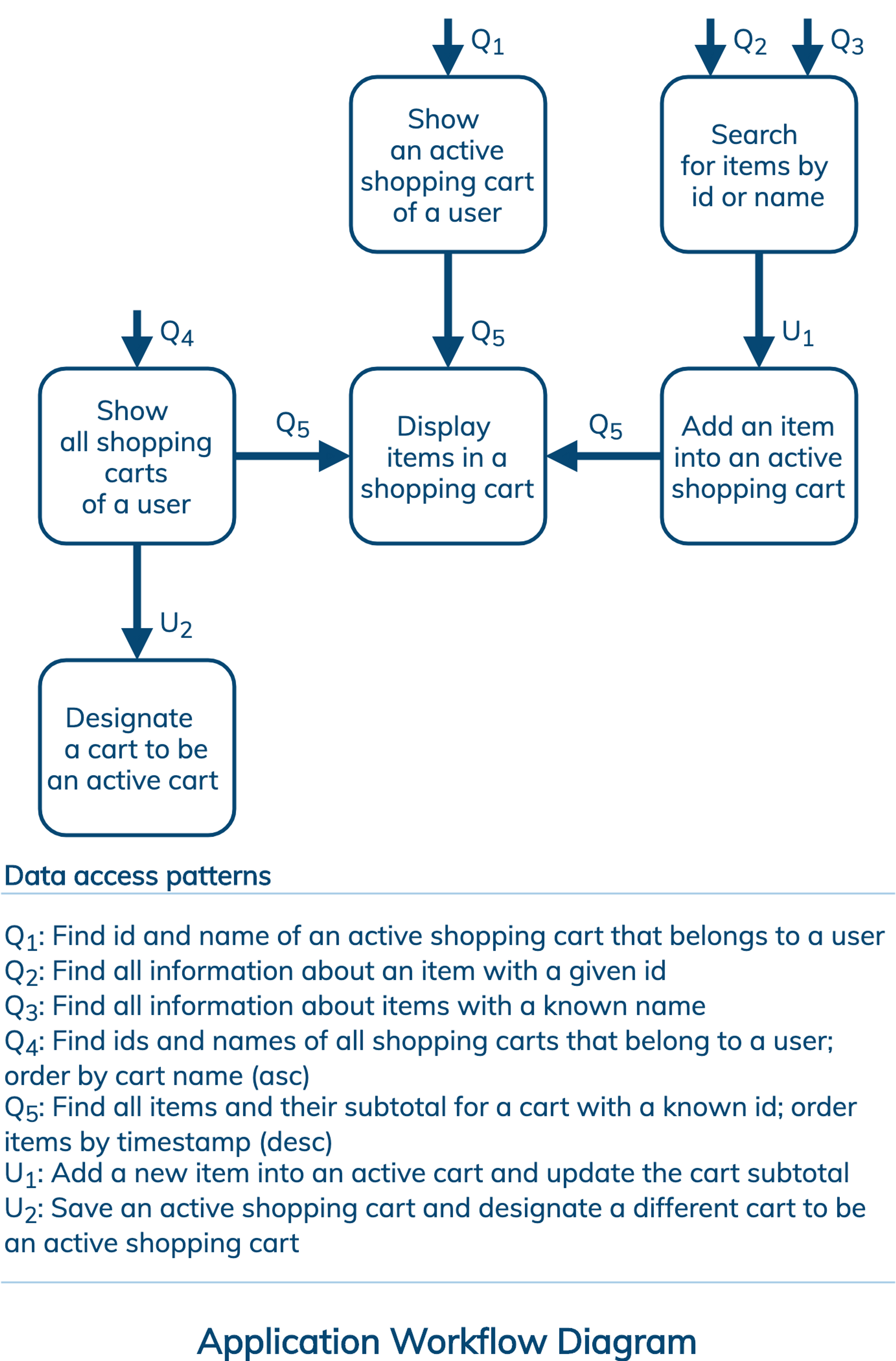
An application workflow is designed with the goal of understanding data access patterns for a data-driven application. Its visual representation consists of application tasks, dependencies among tasks, and data access patterns. Ideally, each data access pattern should specify what attributes to search for, search on, order by, or do aggregation on.
The application workflow has six tasks, of which three tasks are possible entry-point tasks. Based on this workflow, an application should be able to:
- show an active shopping cart of a user, which requires Q1;
- search for items by id or name, which requires Q2 and Q3, respectively;
- show all shopping carts of a user, which requires Q4;
- display items in a shopping cart, which requires Q5;
- add an item into an active shopping cart, which requires U1;
- designate a cart to be an active cart, which requires U2.
All in all, there are seven data access patterns for a database to support. While Q1, Q2, Q3, Q4 and Q5 are needed to query data, U1 and U2 are intended to update data. In this example, updates are especially interesting because they require updating multiple rows and may involve race conditions.
Next: Logical Data Model


Logical Data Model
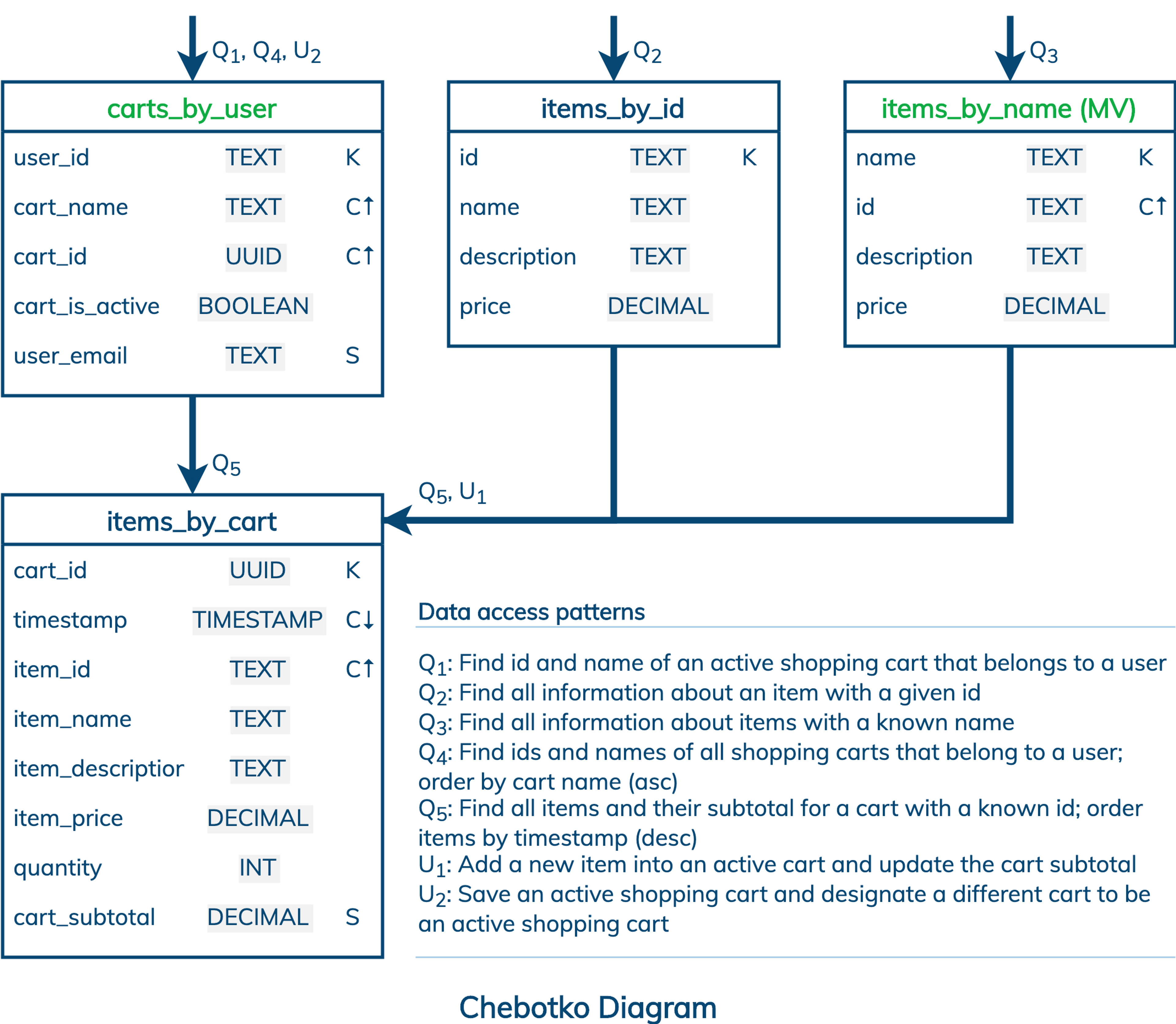
A logical data model results from a conceptual data model by organizing data into Cassandra-specific data structures based on data access patterns identified by an application workflow. Logical data models can be conveniently captured and visualized using Chebotko Diagrams that can feature tables, materialized views, indexes and so forth.
The logical data model for shopping cart data is represented by the shown Chebotko Diagram. Table active_carts_by_user is designed to support data access pattern Q1. It has single-row partitions since each user can only have one active shopping cart at any time. Table items_by_id is designed to support data access pattern Q2. Similarly, it is a table with single-row partitions and a simple primary key. The remaining three tables have multi-row partitions and compound primary keys that consist of both partition and clustering keys. Table items_by_name enables data access pattern Q3. To retrieve all items with a given name, at most one partition needs to be accessed. Next, table all_carts_by_user is designed to support data access pattern Q4. It features one multi-row partition per user, where each row represents a different shopping cart. Rows within each partition are ordered using cart names and cart ids. Column user_email is a static column as it describes a user who is uniquely identified by the table partition key. Again, only one partition in this table needs to be accessed to answer Q4. Finally, table items_by_cart covers data access pattern Q5. In this table, each partition corresponds to a shopping cart and each row represents an item. Column subtotal is a static column and is a descriptor of a shopping cart. Once again, this very efficient design requires retrieving only one partition to satisfy Q5.
Note that, in this example, updates U1 and U2 do not directly affect the table design process. The diagram simply documents which tables need to be accessed to satisfy these data access patterns.
Next: Physical Data ModelPhysical Data Model
A physical data model is directly derived from a logical data model by analyzing and optimizing for performance. The most common type of analysis is identifying potentially large partitions. Some common optimization techniques include splitting and merging partitions, data indexing, data aggregation and concurrent data access optimizations.
The physical data model for shopping cart data is visualized using the Chebotko Diagram. This time, all table columns have associated data types. It should be evident that none of the tables can have very large partitions. Otherwise, some reasonable limits can be enforced by an application, such as at most 100 shopping carts per user, at most 1000 items per cart and at most 10000 items with the same name. The first optimization that this physical data model implements is the elimination of table active_carts_by_user completely and renaming of table all_carts_by_user to simply carts_by_user. The huge advantage of the new design is that U2 becomes much simpler and more efficient to implement because this data access pattern no longer needs to update rows in two tables. In fact, U2 only needs to update two rows in the same partition of table carts_by_user, which can be done efficiently using a batch and a lightweight transaction (see the Skill Building section for a concrete example). The minor disadvantage is that Q1 is not fully supported by table carts_by_user. An application has to retrieve all carts that belong to a user as in Q4 and further scan the result to find an active cart. Assuming that an average user only has a few carts, this should not be a problem at all. Alternatively, it is also possible to create a secondary index on column cart_is_active to fully support Q1 in Cassandra. But using an index to find one row in a partition with only a few rows is likely to be less efficient than simply scanning those few rows (and avoiding index maintenance costs, too). The second and last optimization is the replacement of table items_by_name with a materialized view items_by_name. This is done for convenience rather than efficiency. Our final blueprint is ready to be instantiated in Cassandra.
Skill Building
Skill Building
Want to get some hands-on experience? Give our interactive lab a try! You can do it all from your browser, it only takes a few minutes and you don’t have to install anything.
More Resources
Review the Cassandra data modeling process with these videos