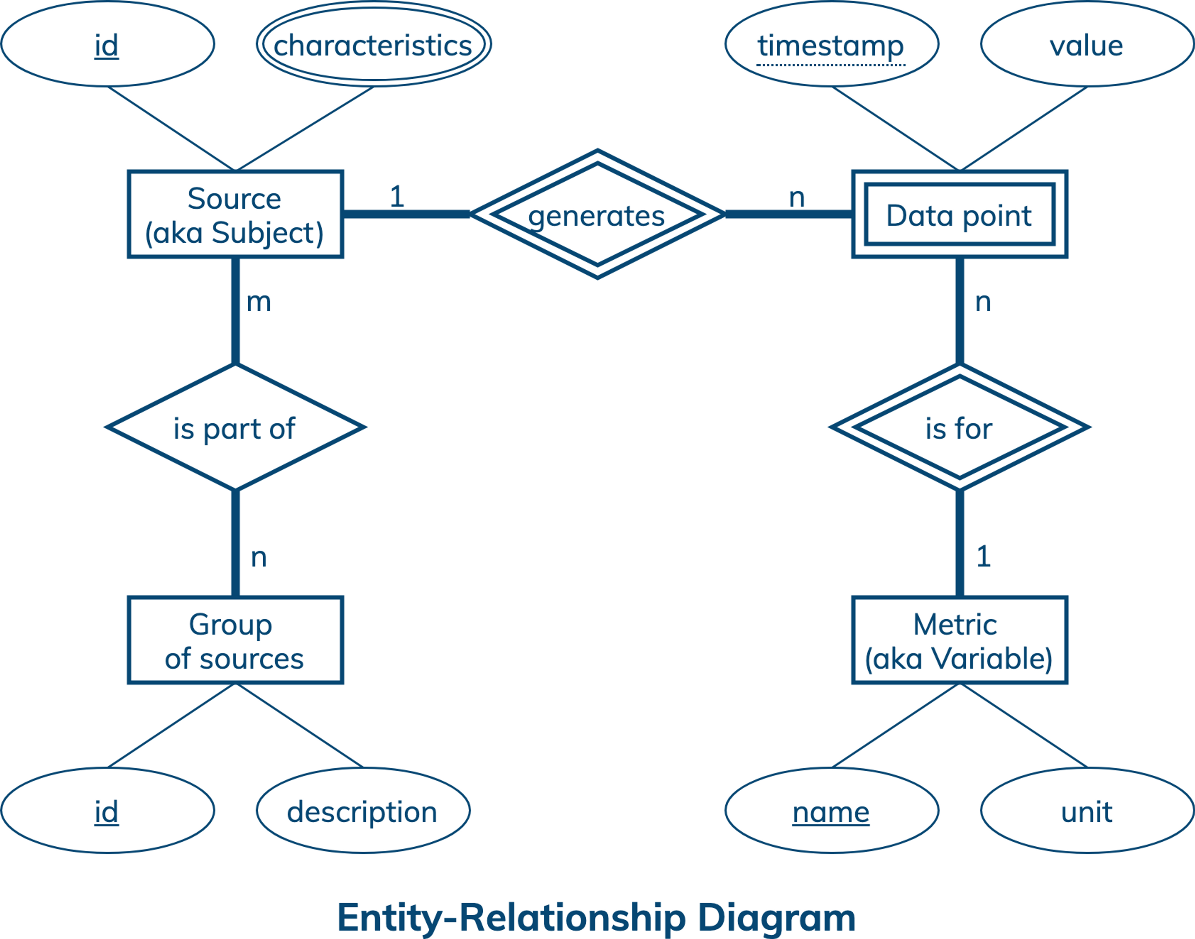
A conceptual data model is designed with the goal of understanding data in a particular domain. In this example, the model is captured using an Entity-Relationship Diagram (ERD) that documents entity types, relationship types, attribute types, and cardinality and key constraints.

A time series is a sequence of data points taken at successive and usually equally spaced out points in time. A time series is generated by a source or collected from a subject and is for a metric or variable. In the diagram, the conceptual data model for time series features data sources, groups of related sources, metrics and data points. Each data source has a unique id and various source-specific characteristics. A group has a unique id and may have a description. A metric is uniquely identified by a metric name and has a unit of measurement. A data point has a timestamp and value, and is uniquely identified by a source id, metric name and data point timestamp. Related data sources can be conveniently organized into groups, where a source can be part of many groups and a group can have many sources. While a source can generate many data points, each data point is collected from only one source. Similarly, there can be many data points for a metric but each data point is for only one metric.

This conceptual data model is generic enough to demonstrate important concepts of time series in Internet of Things applications. It is also simple enough to adapt for many real-life use cases. To make it more evident, let’s consider these examples. First, a sensor network (group) uses sensors (sources) to collect information about temperature, humidity, wind, rainfall, smoke and solar radiation (metrics) for early forest fire detection and monitoring. Second, a smart home (group) uses smart thermostats and appliances (sources) to collect information about temperature, humidity and occupancy (metrics) to optimize energy consumption. Finally, a person (group) uses wearables and medical devices (sources) to collect information about body temperature, blood pressure and heart rate (metrics) to warn about and monitor certain health conditions.

An application workflow is designed with the goal of understanding data access patterns for a data-driven application. Its visual representation consists of application tasks, dependencies among tasks, and data access patterns. Ideally, each data access pattern should specify what attributes to search for, search on, order by, or do aggregation on.

The application workflow has two entry-point tasks. The first entry-point task uses data access pattern Q1 to show all data sources from a particular group. The second entry-point task uses data access pattern Q2 to show all existing metrics. Next, an application has three options: explore time series by source using Q3 and Q4; explore time series by metric using Q5 and Q6; and explore statistics for a time series uniquely identified by a source and a metric using Q7. Data access patterns Q3-Q7 exhibit important characteristics that are common in time series retrieval and analysis:

• Retrieve data based on source (Q3,Q4), metric (Q5,Q6,) or both (Q7);
• Retrieve data based on time range (Q3-Q7);
• Retrieve data using multiple precision or resolution parameters, such as a data point per 60 seconds (Q3,Q5) and a data point per 60 minutes (Q4,Q6);
• Retrieve more recent data with higher resolution (Q3,Q5), because recent data is usually more important and more frequently accessed and analysed;
• Retrieve multiple time series (Q3-Q6) for multi-dimensional analysis;
• Retrieve aggregated data and statistics (Q7).

All in all, there are seven data access patterns for a database to support.

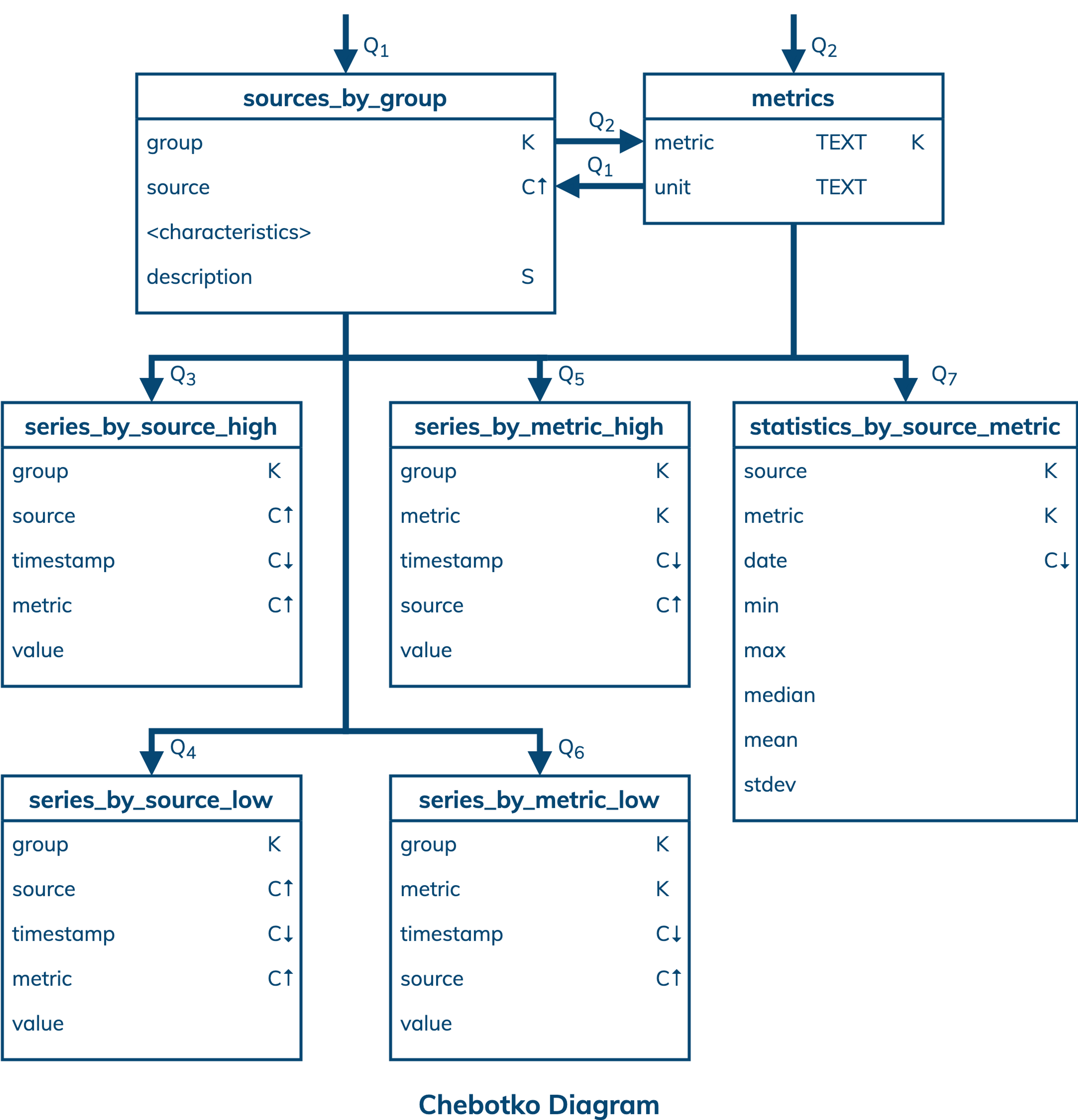
A logical data model results from a conceptual data model by organizing data into Cassandra-specific data structures based on data access patterns identified by an application workflow. Logical data models can be conveniently captured and visualized using Chebotko Diagrams that can feature tables, materialized views, indexes and so forth.

The logical data model for time series data is represented by the shown Chebotko Diagram. There are seven tables, each one supporting a unique data access pattern. Tables sources_by_group and metrics are classic examples of tables with multi-row and single-row partitions, respectively. The former nests all sources belonging to a group as rows in a single partition and uses a static column to describe the group. The latter stores each metric in a separate partition. The remaining five tables demonstrate the three common approaches to organizing time series data: (1) modeling by data source; (2) modeling by metric; and (3) modeling by both data source and metric. Tables series_by_source_high and series_by_source_low demonstrate the first approach. While the table structures are identical, they are intended for time series with different resolutions and can support different data access patterns - Q3 and Q4, respectively. Tables series_by_metric_high and series_by_metric_low are examples of the second approach. Similarly, while the tables have identical structures, they are designed to support different data access patterns - Q5 and Q6, respectively. Finally, table statistics_by_source_metric is a representative of the last approach. It is designed to support data access pattern Q7 and store aggregated data for a time series per partition. In a sense, aggregated data is also a time series with the resolution of 1 day.

Besides the three approaches to time series data modeling, several additional observations can be made. First, multiple time series resolutions result in multiple tables. Second, a mechanism to aggregate data outside of Cassandra is required. Apache Spark™ would be a good choice to compute aggregates. Last, a mechanism to purge older data (e.g., Q3 and Q5 only need 10 days worth of data from the respective tables) is needed. While expiring data with TTL in Cassandra may be convenient, resulting tombstones can slow down reads. Instead, copying only time-relevant data into new tables every once in a while and dropping the old tables could be a better solution. Again, Apache Spark™ would be a good choice for this purpose.

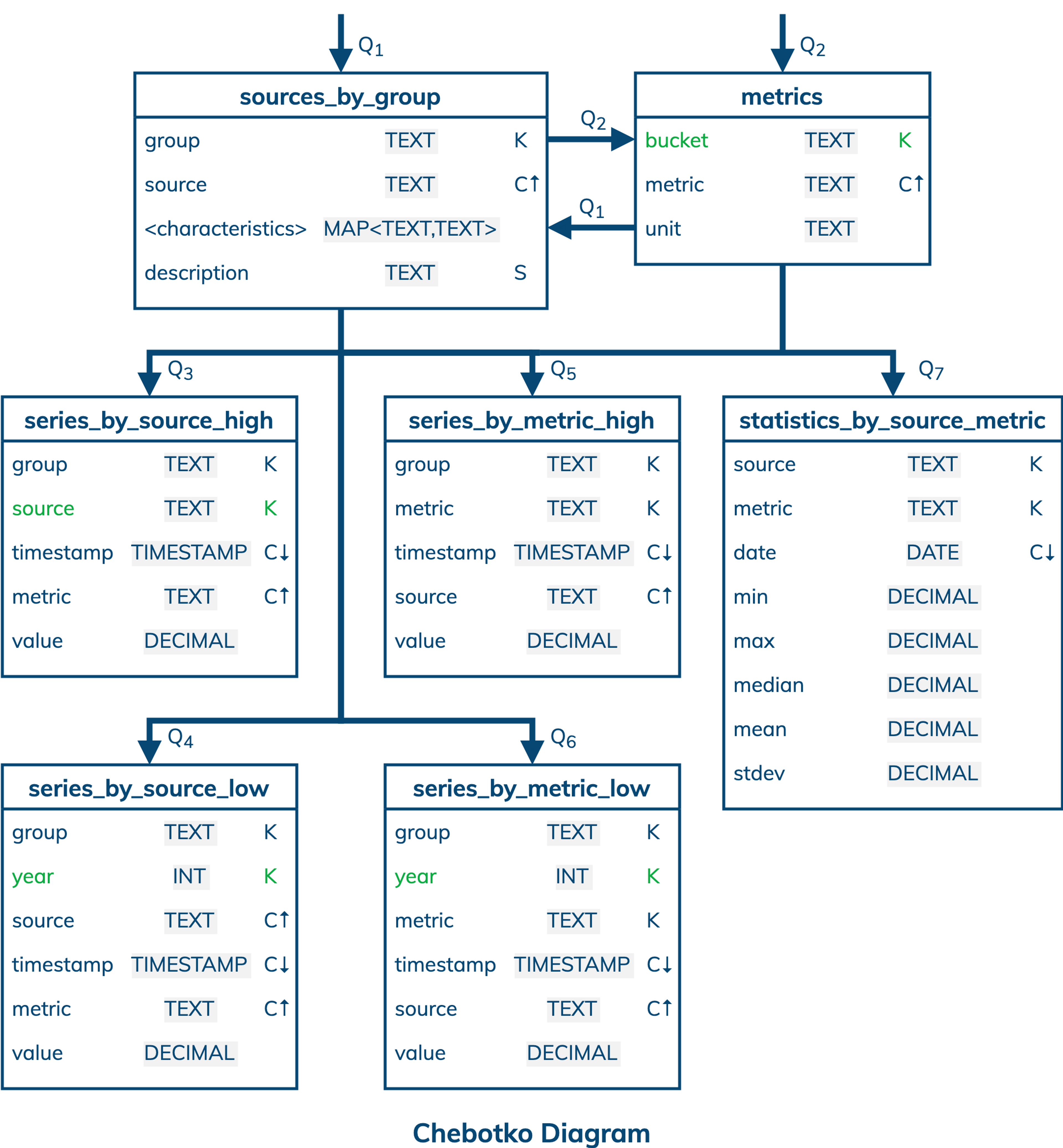
A physical data model is directly derived from a logical data model by analyzing and optimizing for performance. The most common type of analysis is identifying potentially large partitions. Some common optimization techniques include splitting and merging partitions, data indexing, data aggregation and concurrent data access optimizations.

The physical data model for time series data is visualized using the Chebotko Diagram. This time, all table columns have associated data types. In addition, four tables have changes in their primary keys. Table metrics used to be partitioned based on column metric and is now partitioned based on column bucket. The old design had single-row partitions and required retrieving rows from multiple partitions to satisfy Q2. The new design essentially merges old single-row partitions into one multi-row partition and results in much more efficient Q2. The remaining three optimizations applied to tables series_by_source_high, series_by_source_low and series_by_metric_low are all about splitting potentially large partitions. To analyze partition sizes, let’s introduce some assumptions and constraints. Consider that a group can have at most 5 data sources, where each source can generate time series for at most 3 metrics. In other words, all sources in a group can generate 5 x 3 = 15 time series or less. 10 days worth of data from 15 time series with the 60 second resolution each would result in 60 x 24 x 10 x 15 = 216000 data points. With the original design of table series_by_source_high, 216000 data points would be equivalent to 216000 rows in a partition. By making column source a partition key column, the largest partition in table series_by_source_high can have at most 60 x 24 x 10 x 3 = 43200 rows, which is better for performance. The disadvantage of the new design is that Q3 must access multiple partitions when time series from multiple sources are queried. Finally, even though tables series_by_source_low and series_by_metric_low store time series with a low resolution of 60 minutes, these tables collect and retain data for potentially many years. By adding column year as a partition key column, the new design ensures manageable partition sizes. In particular, a partition in table series_by_source_low can have at most 24 x 365 x 15 = 131400 rows for a non-leap year. A partition in table series_by_metric_low can have at most 24 x 365 x 5 = 43800 rows for a non-leap year. Splitting partitions by year is also a good choice with respect to data access patterns Q4 and Q6, where a time range can span at most one year. This way, Q4 or Q6 can always be answered by accessing only one or two partitions. Our final blueprint is ready to be instantiated in Cassandra.

Notice how the assumptions of 5 data sources, 3 metrics and 15 time series per group, which may be suitable for the use cases of smart homes and personal wearables, had a profound impact on the physical data model. Different assumptions (e.g., 1000 sources per group or 1000 sensors per sensor network) may require additional performance optimizations and changes to the data model.